The nowcasting workflow 1: hospital-acquired infections in Bucaramanga, Colombia

This article is an end-to-end walk-through of the tbl.now workflow on a real-life, deliberately messy dataset. We will:

Build a tbl_now from a messy surveillance extract and show how to diagnose() possible data errors.
Clean what it reported: duplicate records, missing dates, etc.
Look at the data with autoplot(), and the summary() functions.
Describe the behaviour of the reporting delay.
Attach temporal effects to a model using the data.
Nowcast with two different engines using everything we found.

We’ll start the process by nowcasting with two dates (event and report dates). We suggest following this example first and then moving to the nowcasting with revisions article if your data also contains revisions (i.e. cases can become ‘confirmed’ or ‘retracted’).

Let’s start by calling the libraries:

library(dplyr)
library(lubridate)
library(ggplot2)
library(tbl.now)

The data

hai_bucaramanga is a raw line list of healthcare-associated infections (IAAS, Infecciones Asociadas a la Atención en Salud) notified in the county of Bucaramanga, Sandander, Colombia, as published by the county. Each row is one infection: a specimen taken from a hospitalised patient, the laboratory result, and the microorganism isolated.

data(hai_bucaramanga)

hai_bucaramanga

#> # A tibble: 6 × 13
#>      id specimen_date received_date report_date specimen    test          microorganism          sex   age_group case_type  final_condition icu_type institution
#>   <int> <date>        <date>        <date>      <fct>       <fct>         <chr>                  <fct> <ord>     <fct>      <fct>           <fct>          <int>
#> 1  1318 2023-01-19    NA            2023-01-22  Whole blood Blood culture Pseudomonas aeruginosa Male  40-49     Laborator… Alive           Adult              1
#> 2  1319 2023-01-24    NA            2023-01-28  Urine       Urine culture Serratia marcescens    Male  60-69     Laborator… Alive           Adult              1
#> 3  1320 NA            NA            NA          NA          NA            NA                     Male  70+       Clinicall… Alive           Adult              5
#> 4  1321 2023-01-29    NA            2023-01-31  Urine       Urine culture Klebsiella pneumoniae  Male  60-69     Laborator… Alive           Adult              1
#> 5  1322 2023-01-19    NA            2023-01-20  Urine       Urine culture Escherichia coli       Male  70+       Laborator… Alive           Adult              6
#> # ℹ 1 more row

For our example, six columns matter:

id — a unique patient identifier.
specimen_date — the event date, when the sample was taken.
report_date — the report date, when the laboratory issued the result.
sex - the sex of the individual.

For the tutorial, we will do perform a nowcast assuming we are standing on July 18th 2022. For that purpose we filter our data to what it would have looked like back then:

hai_bucaramanga <- hai_bucaramanga |>
  filter((is.na(specimen_date) | specimen_date <= ymd("2022/07/18")), 
         (is.na(report_date)   | report_date   <= ymd("2022/07/18")))

For this tutorial we are keeping those events that have missing dates to show how to detect them with the package. That is what the is.na() section on the left side of the filter is doing.

1. Initial data cleaning

In this tutorial we show how to discover several anomalies in the data as well as several modeling indicators. We suggest, however, that before transforming the dataset into a tbl_now you use traditional data analysis tools to clean the data first. Here we’ll just select the columns that matter to us and move onto the tbl_now capabilities. However if you already have a pipeline for cleaning and preparing your data this is where you would do it as we’ll see the tbl_now diagnostics don’t cover everything.

#We keep only the columns of interest
hai_bucaramanga <- hai_bucaramanga |> 
  select(id, specimen_date, report_date, sex)

2. Building the `tbl_now`

We’ll create the tbl_now() object. For the beginning of the example, we will declare two dates (specimen_date for the event and report_date) for the report. We’ll further specify that the data is in line-list format (i.e. each row is a case), and stratify by sex.

hai_bucaramanga <- hai_bucaramanga |>
  tbl_now(
    event_date   = specimen_date,
    report_date  = report_date,
    strata       = sex,
    data_type    = "linelist",
    event_units  = "days",
    report_units = "days"
  )
#> Warning: 363 rows have NA values in the report_date column "report_date".
#> ℹ A row with no report date cannot be placed on the reporting triangle.
#> Warning: 314 rows have NA values in the event_date column "specimen_date".
#> ℹ A row with no event date cannot be placed on the reporting triangle.
#> Warning: 48 rows have a `report_date` before `event_date`
#> ℹ A negative reporting delay is not a delay; the two date columns may be swapped, or the rows may be data-entry errors.
#> Warning: 304 rows have NA values in the event and report date columns: "specimen_date" and "report_date".
#> ℹ

The tbl.now() automatically fires several warnings. Let’s take a look!

The tbl.now() package also considers the possibility of a third revision_date where reports that have already been submitted by report_date are either confirmed or rejected (or maybe just one of those). We show more diagnostics for such an example in its own article though we suggest familiarizing yourself with this one first.

3. What is wrong?

These same warnings can also be accessed with the diagnose() function which returns the warnings as well as additional notes:

diagnose(hai_bucaramanga) 
#> ── Diagnosis of a <tbl_now> ────────────────────────────────────────────────────────────────────────────────────────────────────────────────────────────────────
#> 4 warnings, 8 notes, 12 passed, 5 skipped.
#> 
#> Warnings (4)
#> ! missing/report_date: 363 rows have NA values in the report_date column "report_date".
#>   → A row with no report date cannot be placed on the reporting triangle.
#> ! missing/specimen_date: 314 rows have NA values in the event_date column "specimen_date".
#>   → A row with no event date cannot be placed on the reporting triangle.
#> ! ordering/event_to_report: 48 rows have a `report_date` before `event_date`
#>   → A negative reporting delay is not a delay; the two date columns may be swapped, or the rows may be data-entry errors.
#> ! simultaneously missing/event and report dates: 304 rows have NA values in the event and report date columns: "specimen_date" and "report_date".
#>   → 
#> 
#> Notes (8)
#> ℹ declarations/undeclared: 1 column "id" is not declared as strata or covariates.
#>   → Declare it with `strata = ` to model it separately, or let `to_count()` pool it away -- which is what the `tbl_now_to_()` converters do.
#> ℹ now/now_gap_event [Female]: The last event date is 32 days before now ("2022-07-18").
#>   → Everything in that window is still arriving; it is what a nowcast is for, and it is also what makes the last points of any plot look like a decline.
#> ℹ now/now_gap_report [Female]: The last report date is 10 days before now ("2022-07-18").
#> ℹ strata/size [Female]: The smallest stratum is "Female" with 329 cases, 38.6% of the total.
#> ℹ strata/sparsity [Female]: The sparsest stratum is "Female": 768 of the 929 days between the minimum event (NA) and the now (2022-07-18) carry no cases at all (82.7%, against 63% pooled over every stratum).
#>   → A stratum that is mostly zeros is the one a per-stratum fit will struggle with; pooling it is often better than fitting it. When every stratum is mostly zeros the grid is finer than the data -- `aggregate_time_units()` coarsens it.
#> ℹ truncation/event_date [Female]: 10 event dates are younger than the 95th percentile of the delay, so their counts are still filling in; an estimated 10.6% of their eventual total has not arrived.
#>   → This is right-truncation, and it is the reason to nowcast rather than a defect. Cut the series at "2022-03-20" to describe it instead.
#> ℹ truncation/event_date [Male]: 15 event dates are younger than the 95th percentile of the delay, so their counts are still filling in; an estimated 25.5% of their eventual total has not arrived.
#> ℹ truncation/event_date: 24 event dates are younger than the 95th percentile of the delay, so their counts are still filling in; an estimated 20.5% of their eventual total has not arrived.
#> 
#> ✔ 12 passed: declarations/temporal_effects, missing/sex, now/event_date, now/now_gap_event, now/now_gap_report, now/report_date, units/declared, units/delay, units/event_grid, and units/report_grid
#> ─ 5 skipped: duplicates/key, negatives/count, ordering/event_to_revision, ordering/report_to_revision, and strata/pending
#> 
#> ℹ 29 findings. Use `dplyr::filter()` or `tibble::as_tibble()` for the table.

Let’s see what they identify.

The warnings

In general the warnings will look for missing data within the dates and the strata or for violations of the nowcasting hypotheses (for example reports that “see the future” and identify an event before it happens!). In our case, specifically we identify missing dates in both the report and the event as well as some reports that have incorrect dates.

There is no solution that works in all cases for these problems and oftentimes the ideal solution is to identify the reason for the misingness. Here we posit some approaches for the warnings:

For simultaneosuly missing event and report dates there is nothing one can do. In those cases we don’t know when something happened (to add to the epidemic process) or when it was reported (to add to the delay process). Hence we remove those rows.

#Remove those that have both dates missing
hai_bucaramanga <- hai_bucaramanga |> 
  filter(!(is.na(report_date) & is.na(specimen_date)))

For the rows with missing reports, we can censor them above. This will tell the models in diseasenowcasting that the measurement is not exact; instead, that we know the report arrived before a certain date though we don’t know that exact date in particular. We can do this because if we are seeing the reports today then we know that at most they took until today to arrive. This censoring will add a column .is_censored_report which will indicate that that report is censored.

When calling the function we specify that the ones we are censoring are the missing values and that the date they should input is "2022/10/18" which corresponds to the date of the nowcast in this example.

hai_bucaramanga <- hai_bucaramanga |> 
  censor_reports(is.na(report_date), to_report = as.Date("2022/07/18"))

For the delays before the reports we visualize the data. Doing a quick analysis we see that its a date formatting issue. You can see in the first entries that the specimen date is in format year-day-month (read with lubridate::ydm()) while the report_date and received_date is in format year-month-day (read with lubridate::ymd()) .

hai_bucaramanga |> filter(report_date < specimen_date) 
#> # A tibble:  48 × 8
#> # Data type: "linelist"
#> # Frequency: Event: `days` | Report: `days`
#>      id specimen_date report_date   sex      .is_censored_report  .event_num .report_num .delay
#>   <int> <date>        <date>        <fct>    <lgl>                     <dbl>       <dbl>  <dbl>
#>   [...] [event_date]  [report_date] [strata] [is_censored_report]      [...]       [...]  [...]
#> 1   590 2020-11-07    2020-07-21    Female   FALSE                       310         201   -109
#> 2   613 2020-10-08    2020-08-13    Male     FALSE                       280         224    -56
#> 3   622 2020-08-28    2020-01-09    Male     FALSE                       239           7   -232
#> 4   623 2020-08-28    2020-03-09    Female   FALSE                       239          67   -172
#> 5   626 2020-08-30    2020-02-09    Female   FALSE                       241          38   -203
#> # ────────────────────────────────────────────────────────────────────────────────────────────────────────────────────────────────────────────────────────────────
#> # Now: 2022-07-18 | Event date: "specimen_date" | Report date: "report_date"
#> # left-censored indicator: ".is_censored_report"
#> # Strata: "sex"
#> # ────────────────────────────────────────────────────────────────────────────────────────────────────────────────────────────────────────────────────────────────
#> # ℹ 43 more rows

We can correct the date format to fix this issue:

hai_bucaramanga <- hai_bucaramanga |> 
  mutate(specimen_date = if_else(specimen_date > report_date, 
                                 ydm(as.character(specimen_date)), 
                                 ymd(as.character(specimen_date))))

Currently there is nothing we can do for the cases were the event date is unknown. Hence we just document them and we’ll remove from the dataset given that they represent such a small percent (5.7%).

hai_bucaramanga <- hai_bucaramanga |> filter(!is.na(specimen_date))

Re-running diagnose() confirms we solved this issues:

diagnose(hai_bucaramanga)
#> ── Diagnosis of a <tbl_now> ────────────────────────────────────────────────────────────────────────────────────────────────────────────────────────────────────
#> 7 notes, 20 passed, 5 skipped.
#> 
#> Notes (7)
#> ℹ declarations/undeclared: 1 column "id" is not declared as strata or covariates.
#>   → Declare it with `strata = ` to model it separately, or let `to_count()` pool it away -- which is what the `tbl_now_to_()` converters do.
#> ℹ now/now_gap_event [Female]: The last event date is 32 days before now ("2022-07-18").
#>   → Everything in that window is still arriving; it is what a nowcast is for, and it is also what makes the last points of any plot look like a decline.
#> ℹ strata/size [Female]: The smallest stratum is "Female" with 195 cases, 37.7% of the total.
#> ℹ strata/sparsity [Female]: The sparsest stratum is "Female": 777 of the 929 days between the minimum event (2020-01-02) and the now (2022-07-18) carry no cases at all (83.6%, against 64.5% pooled over every stratum).
#>   → A stratum that is mostly zeros is the one a per-stratum fit will struggle with; pooling it is often better than fitting it. When every stratum is mostly zeros the grid is finer than the data -- `aggregate_time_units()` coarsens it.
#> ℹ truncation/event_date [Female]: 140 event dates are younger than the 95th percentile of the delay, so their counts are still filling in; an estimated 76.8% of their eventual total has not arrived.
#>   → This is right-truncation, and it is the reason to nowcast rather than a defect. Cut the series at "2020-05-01" to describe it instead.
#> ℹ truncation/event_date [Male]: 204 event dates are younger than the 95th percentile of the delay, so their counts are still filling in; an estimated 71.7% of their eventual total has not arrived.
#> ℹ truncation/event_date: 300 event dates are younger than the 95th percentile of the delay, so their counts are still filling in; an estimated 74.7% of their eventual total has not arrived.
#> 
#> ✔ 20 passed: declarations/temporal_effects, missing/.is_censored_report, missing/report_date, missing/sex, missing/specimen_date, now/event_date, now/now_gap_event, now/now_gap_report, now/report_date, ordering/event_to_report, simultaneously missing/event and report dates, units/declared, units/delay, units/event_grid, and units/report_grid
#> ─ 5 skipped: duplicates/key, negatives/count, ordering/event_to_revision, ordering/report_to_revision, and strata/pending
#> 
#> ℹ 32 findings. Use `dplyr::filter()` or `tibble::as_tibble()` for the table.

The notes

The notes convey additinal information that, at a glance, can tell you whether something needs to be corrected in your data.

It helps you know that you have columns that are not strata or covariates (in case you forgot to declare them!):

declarations/undeclared: 3 columns "id", "received_date", and "microorganism" are not declared as strata or covariates.

It quantifies how much time has happened between the last observation and the now for each strata:

now/now_gap_event [Female]: The last event date is 32 days before now ("2022-07-18").

It also tells you how what is the smallest stratum (in case you have strata with so few observations you need to collapse them into another one):

strata/size [Female]: The smallest stratum is "Female" with 195 cases, 37.7% of the total.

And how sparse your data is:

strata/sparsity [Female]: The sparsest stratum is "Female": 777 of the 929 "days" between the minimum event (2020-01-02) and the now (2022-07-18) carry no cases at all (83.6%, against 64.5% pooled over every stratum).

This is particularly useful for triangle-based methods that require to fill with zeroes the whole reporting triangle.

4. More cleaning

Besides the diagnose() one always has to do some additional cleaning of datasets. One particular issue is for repeated rows; that is when an individual is registered twice in the dataset for the same disease at the same exact times.

Here we can see that the same individuals id are sometimes repeated:

hai_bucaramanga |>
  count(id, report_date, specimen_date) |>
  filter(n > 1) |> 
  as_tibble()
#> Warning: Dropping `tbl_now` attributes and converting to `tibble`
#> Warning: Dropped protected column(?s): ".is_censored_report", ".event_num", ".report_num", and ".delay". Returning a
#> `tibble`
#> # A tibble: 18 × 4
#>      id report_date specimen_date     n
#>   <int> <date>      <date>        <int>
#> 1  1225 2022-05-16  2022-05-13        2
#> 2  1226 2022-05-18  2022-05-18        2
#> 3  1227 2022-05-18  2022-05-17        2
#> 4  1228 2022-05-19  2022-05-17        2
#> 5  1229 2022-05-20  2022-05-17        2
#> # ℹ 13 more rows

We can use dplyr::distinct() to remove them without losing information:

hai_bucaramanga <- hai_bucaramanga |> distinct()

5. Temporal effects

Temporal covariates can be added to a tbl_now so that we can describe their effect or use them for nowcasting. They can be specified via the temporal_effects() function. It can add holidays, weekends, day of the week effects and more. For the purpose of this tutorial we will add the weekends and check whether there is a weekend effect or not:

temporal_effects(weekend = TRUE)
#> ── Temporal Effects ────────────────────────────────────────────────────────────────────────────────────────────────────────────────────────────────────────────
#> The following effects are in place:
#> • "weekend"

You can add the effects to the tbl_now() with the add_temporal_effects() function:

hai_bucaramanga <- hai_bucaramanga |> 
  add_temporal_effects(t_effects = temporal_effects(weekend = TRUE))

hai_bucaramanga
#> # A tibble:  499 × 8
#> # Data type: "linelist"
#> # Frequency: Event: `days` | Report: `days`
#>      id specimen_date report_date   sex      .is_censored_report  .event_num .report_num .delay
#>   <int> <date>        <date>        <fct>    <lgl>                     <dbl>       <dbl>  <dbl>
#>   [...] [event_date]  [report_date] [strata] [is_censored_report]      [...]       [...]  [...]
#> 1   528 2020-10-01    2022-07-18    Male     TRUE                        273         928    655
#> 2   529 2020-10-01    2022-07-18    Male     TRUE                        273         928    655
#> 3   530 2020-01-23    2022-07-18    Female   TRUE                         21         928    907
#> 4   531 2020-07-01    2022-07-18    Male     TRUE                        181         928    747
#> 5   532 2020-07-01    2022-07-18    Male     TRUE                        181         928    747
#> # ────────────────────────────────────────────────────────────────────────────────────────────────────────────────────────────────────────────────────────────────
#> # Now: 2022-07-18 | Event date: "specimen_date" | Report date: "report_date"
#> # left-censored indicator: ".is_censored_report"
#> # Strata: "sex"
#> # T. effects (lazy): [event_date] weekend
#> # ────────────────────────────────────────────────────────────────────────────────────────────────────────────────────────────────────────────────────────────────
#> # ℹ 494 more rows

The temporal effect gets added lazily. You can use compute_temporal_effects() to show it as a column in case you require it (see them at the end of the tbl_now).

hai_bucaramanga |> compute_temporal_effects()
#> # A tibble:  499 × 9
#> # Data type: "linelist"
#> # Frequency: Event: `days` | Report: `days`
#>      id specimen_date report_date   sex      .is_censored_report  .event_num .report_num .delay .event_weekend
#>   <int> <date>        <date>        <fct>    <lgl>                     <dbl>       <dbl>  <dbl>          <int>
#>   [...] [event_date]  [report_date] [strata] [is_censored_report]      [...]       [...]  [...]     [t_effect]
#> 1   528 2020-10-01    2022-07-18    Male     TRUE                        273         928    655              0
#> 2   529 2020-10-01    2022-07-18    Male     TRUE                        273         928    655              0
#> 3   530 2020-01-23    2022-07-18    Female   TRUE                         21         928    907              0
#> 4   531 2020-07-01    2022-07-18    Male     TRUE                        181         928    747              0
#> 5   532 2020-07-01    2022-07-18    Male     TRUE                        181         928    747              0
#> # ────────────────────────────────────────────────────────────────────────────────────────────────────────────────────────────────────────────────────────────────
#> # Now: 2022-07-18 | Event date: "specimen_date" | Report date: "report_date"
#> # left-censored indicator: ".is_censored_report"
#> # Strata: "sex"
#> # T. effects: [event_date] weekend
#> # T. effect cols: ".event_weekend"
#> # ────────────────────────────────────────────────────────────────────────────────────────────────────────────────────────────────────────────────────────────────
#> # ℹ 494 more rows

For a deeper explanation on what to see in each of the panels when there are effects and no effects you can see the article on diagnosing a tbl.now

6. Looking at the data

autoplot() draws a diagnostic grid with the panels in green describing the epidemic process and the red ones, the reporting process.

autoplot(hai_bucaramanga)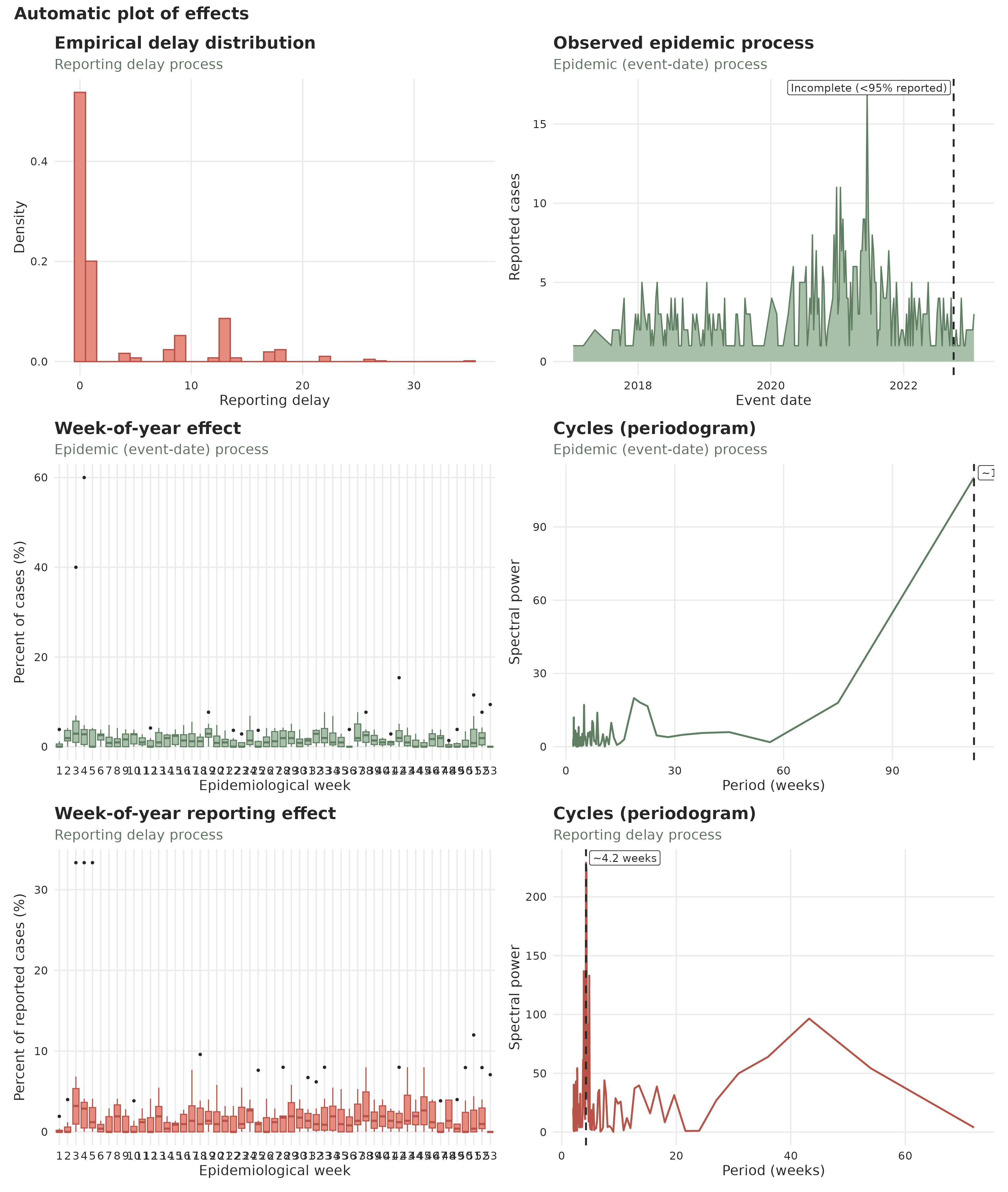

A six-panel diagnostic grid: empirical delay distribution, observed epidemic curve, month-of-year effects for cases and for reporting, and periodograms for both processes.

Four things stand out, and each of them changes a modelling decision later.

The epidemic curve is extremely sparse. There are only a handful of cases a year with most of the times 0 or 1 cases being reported.

plot_epidemic_process(hai_bucaramanga)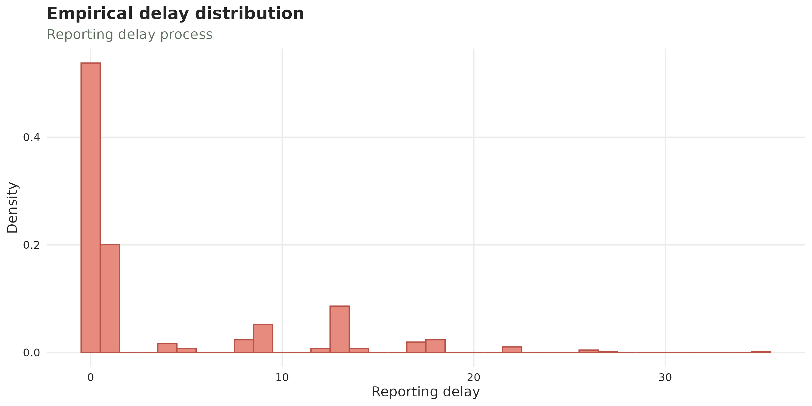

Epidemic process.

Note This is the same sparcity the note in the diagnostic() function gave us.

The delay distribution has some extreme delays. This is the most consequential feature of the dataset, so it is worth its own plot:

plot_delay_distribution(hai_bucaramanga)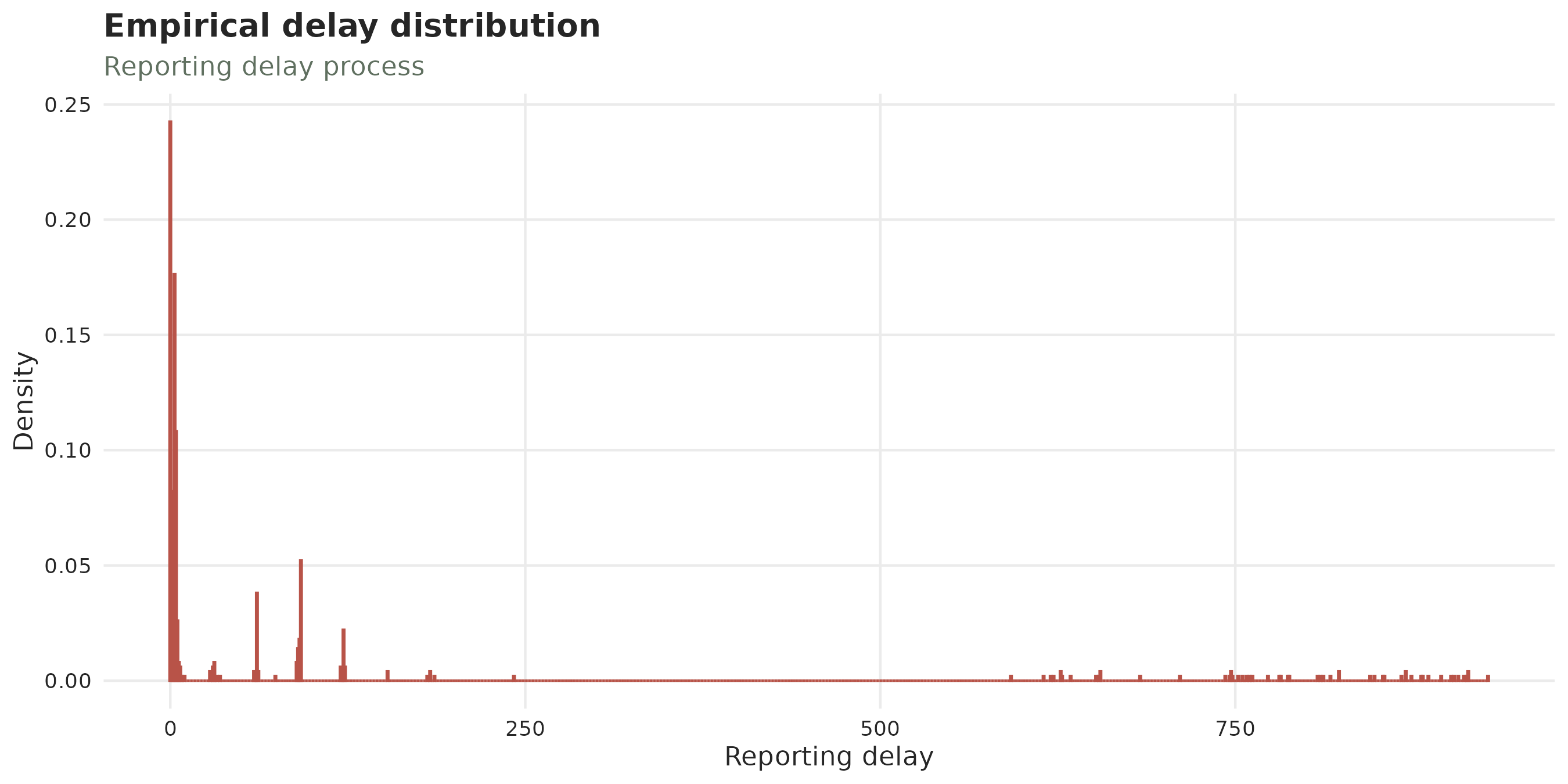

Histogram of the reporting delay.

A lot of results are reported way after 500 days!

There doesn’t seem to be a day-of-the-week effect In both reports and events there is no aparent day of the week effect.

plot_day_of_week_effects(hai_bucaramanga)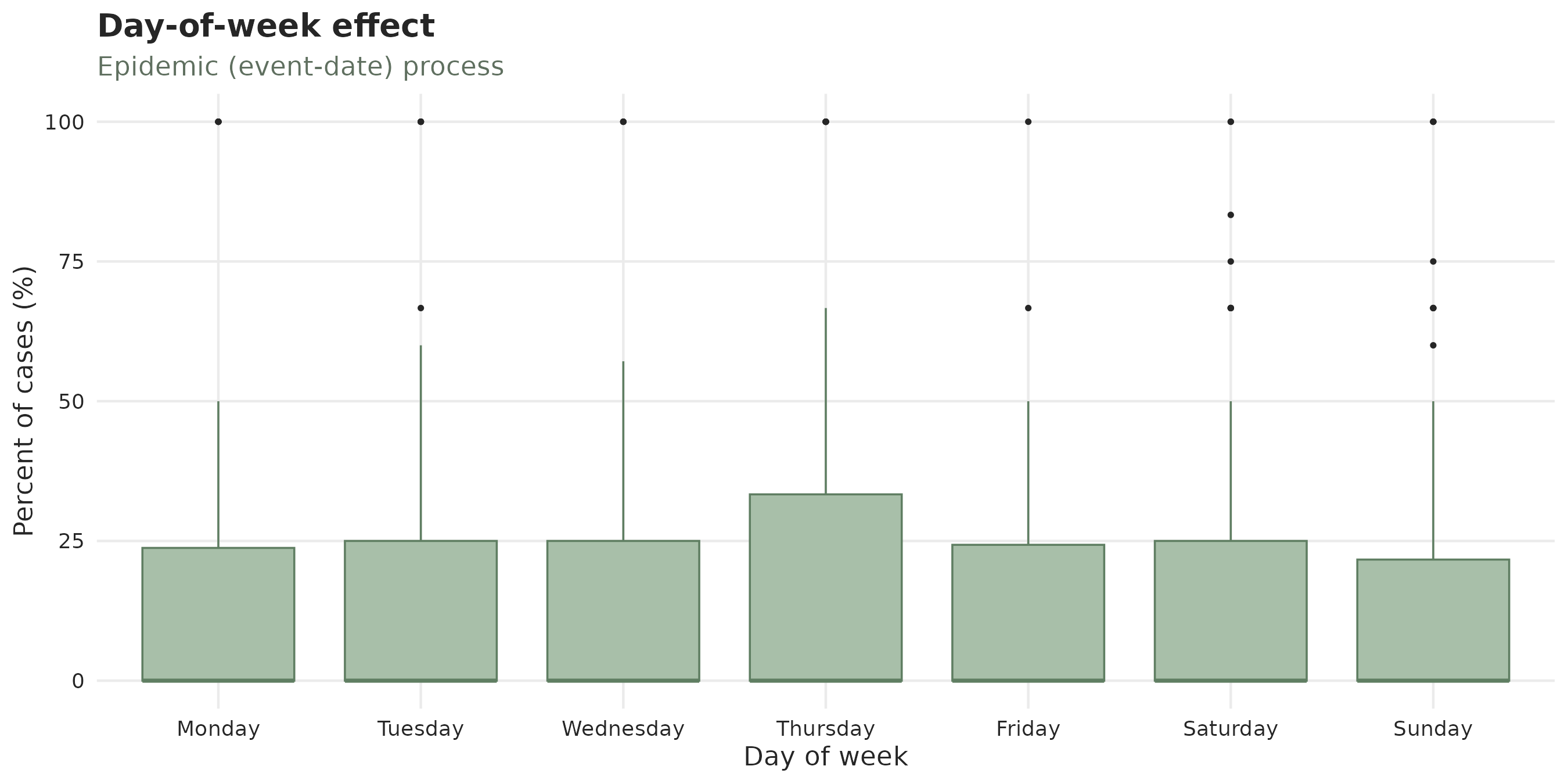

Effects in the week

One week had a lot of reports Epiweek 29 is an anomaly in the amount of reports it seems to have. This would warrant further investigation.

plot_week_of_year_effects(hai_bucaramanga, type = "report")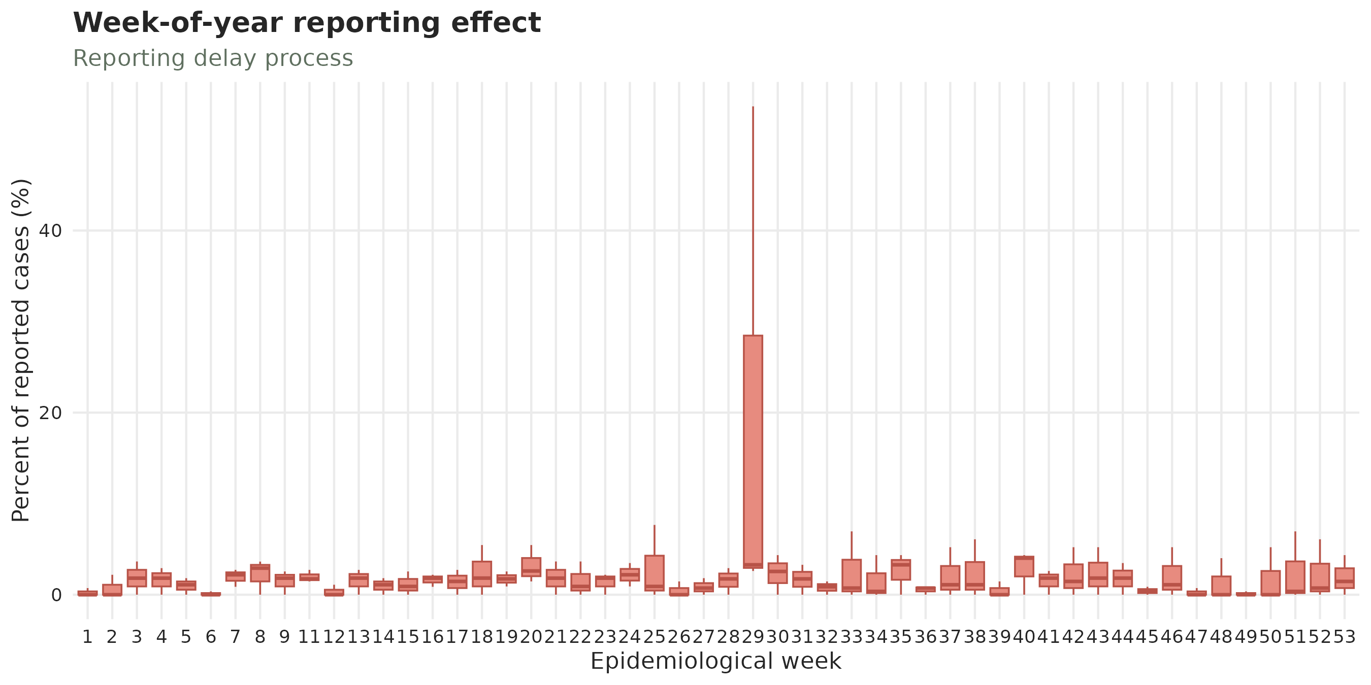

Effects on the report

There doesn’t seem to be a weekend effect either In both reports and events there is no aparent effect of a weekend.

plot_weekend_effects(hai_bucaramanga)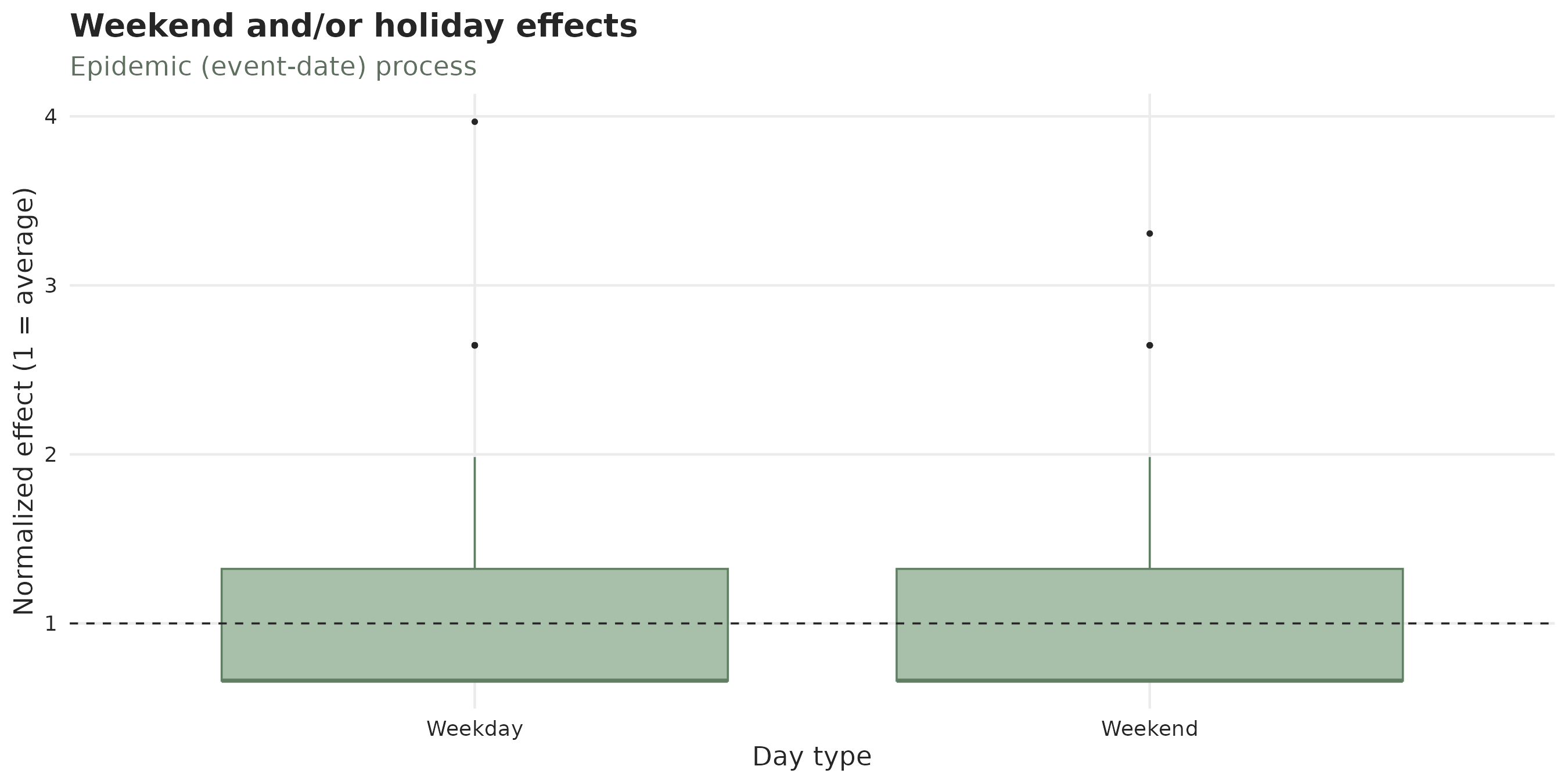

Effects in the week

7. Summarising the data

The summary() of a tbl_now quantifies what we see in the plots. You can either call summary() all at once:

summary(hai_bucaramanga)

or as we do here call each of the summaries we are going to discuss (see ?nowcast_summary_components for the whole list).

We can start with the delays. Here we can see that up until the 3rd quartile (q75) delays are less than 100 days but then they explode by the 90th quantile (q90):

delay_summary(hai_bucaramanga)
#> ── Summary of a <tbl_now> ──────────────────────────────────────────────────────────────────────────────────────────────────────────────────────────────────────
#> 3 rows in 1 component; strata: "Female" and "Male".
#> 
#> delay
#>   n = (event, report) cells; total = cases
#>   quantity        stratum     n total  mean    sd   min   q25   q50   q75   q90   max
#>   <chr>           <chr>   <int> <dbl> <dbl> <dbl> <dbl> <dbl> <dbl> <dbl> <dbl> <dbl>
#> 1 event_to_report all       438   499 107.   243.     0     1     3    89   627   928
#> 2 event_to_report Female    170   188  89.3  228.     0     2     3    35   186   914
#> 3 event_to_report Male      268   311 118.   252.     0     0     4    91   634   928
#> 
#> ℹ Use `dplyr::filter()` or `tibble::as_tibble()` for the full schema.

The zero_run_summary() quantifies the sparcity by counting how many days with continuous zeroes happened for either the event or the report dates. That is, it measures the distribution of days when nothing happened (hence zero registries). You can see that usually there are on average 3.06 days with no cases before one with a case. You can also see that there have been runs of 25 continuous days with no cases (continuous zeroes) until one case:

zero_run_summary(hai_bucaramanga)
#> ── Summary of a <tbl_now> ──────────────────────────────────────────────────────────────────────────────────────────────────────────────────────────────────────
#> 3 rows in 1 component; strata: "Female" and "Male".
#> 
#> zero_run
#>   n = runs of consecutive zero dates; total = zero dates in those runs
#>   quantity   stratum     n total  mean    sd   min   q25   q50   q75   q90   max
#>   <chr>      <chr>   <int> <dbl> <dbl> <dbl> <dbl> <dbl> <dbl> <dbl> <dbl> <dbl>
#> 1 event_date all       196   599  3.06  3.29     1     1     2     4     6    25
#> 2 event_date Female    123   777  6.32  6.31     1     2     4     8    13    32
#> 3 event_date Male      159   703  4.42  4.87     1     1     3     6     9    29
#> 
#> ℹ Use `dplyr::filter()` or `tibble::as_tibble()` for the full schema.

The composition block shows that there are way less females than males. Which, again was already observed in the notes as the smaller stratum:

prop_strata(hai_bucaramanga)
#> ── Summary of a <tbl_now> ──────────────────────────────────────────────────────────────────────────────────────────────────────────────────────────────────────
#> 2 rows in 1 component.
#> 
#> composition
#>   n = (event, report) cells in the category; total = cases in the category
#>   quantity            n total  prop
#>   <chr>           <int> <dbl> <dbl>
#> 1 strata = Female   170   188 0.377
#> 2 strata = Male     268   311 0.623
#> 
#> ℹ Use `dplyr::filter()` or `tibble::as_tibble()` for the full schema.

Finally the cases per date shows how many cases on average occur per date-axis. That is on average how many cases there are per event date or per report date. In this case we can see that at least half of the dates have zero cases:

cases_per_date(hai_bucaramanga)
#> ── Summary of a <tbl_now> ──────────────────────────────────────────────────────────────────────────────────────────────────────────────────────────────────────
#> 6 rows in 1 component; strata: "Female" and "Male".
#> 
#> cases
#>   n = dates on the grid; total = cases
#>   quantity                stratum     n total   mean    sd   min   q25   q50   q75   q90   max prop_zero
#>   <chr>                   <chr>   <int> <dbl>  <dbl> <dbl> <dbl> <dbl> <dbl> <dbl> <dbl> <dbl>     <dbl>
#> 1 per_event_date          all       929   499 0.537  0.877     0     0     0     1     2     6     0.645
#> 2 censored_per_event_date all       929    58 0.0624 0.267     0     0     0     0     0     2     0.944
#> 3 per_event_date          Female    929   188 0.202  0.500     0     0     0     0     1     3     0.836
#> 4 censored_per_event_date Female    929    20 0.0215 0.145     0     0     0     0     0     1     0.978
#> 5 per_event_date          Male      929   311 0.335  0.678     0     0     0     0     1     5     0.757
#> 6 censored_per_event_date Male      929    38 0.0409 0.219     0     0     0     0     0     2     0.963
#> 
#> ℹ Use `dplyr::filter()` or `tibble::as_tibble()` for the full schema.

Intermezzo: The first nowcast

Even with all this sparcity here we can nowcast using the diseasenowcasting package:

hai_fit <- hai_bucaramanga |> 
  run_nowcast(engine = engine_diseasenowcasting(temporal_effects = "none"))
#> ℹ Nowcasting with "diseasenowcasting" as of 2022-07-18.

Due to the sparcity, the nowcast predicts almost no cases at any time with just maybe a second case at the now for males:

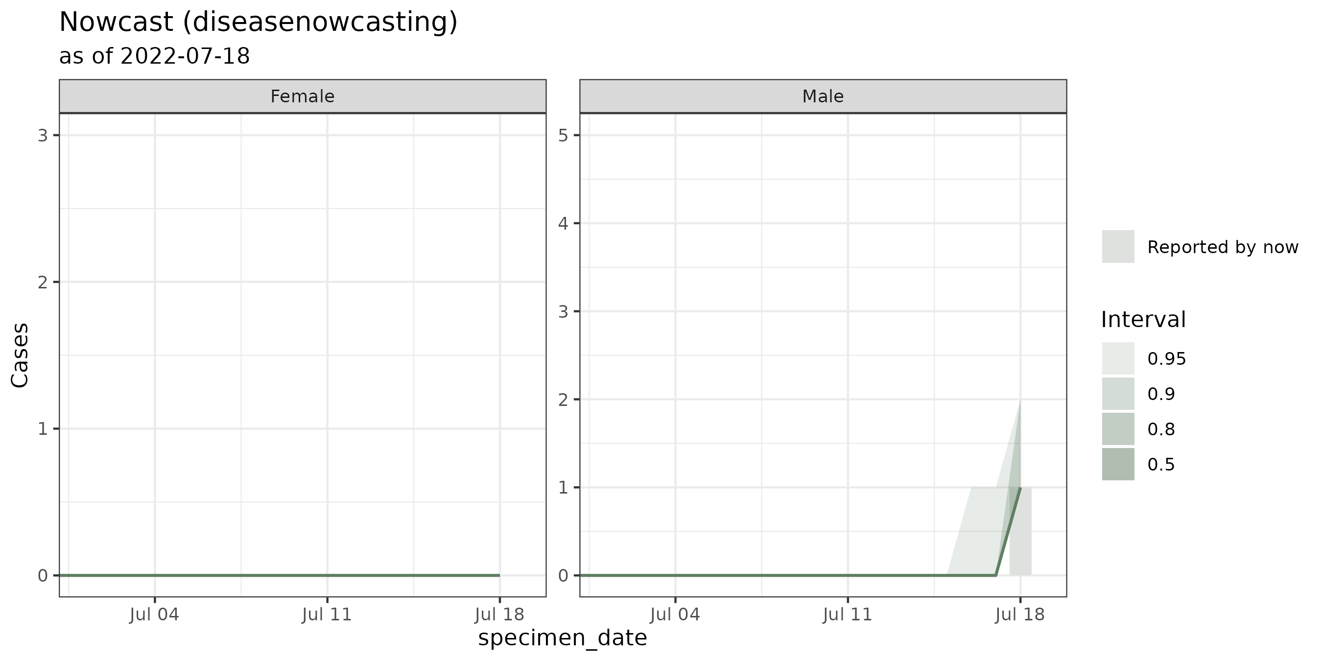
autoplot(hai_fit, date_lim = c(as.Date("2022-07-01"), as.Date("2022-07-19")))

A sparse nowcast

8. Changing to weekly data

Though nowcasting is possible with sparse data, oftentimes people prefer to rescale data to a coarser time frame (and some packages can’t handle the sparcity either). Here we’ll rescale the dataset to a weekly reporting time frame with aggregate_time_units():

hai_bucaramanga <- hai_bucaramanga |> 
  aggregate_time_units(to = "weeks")
#> ℹ Dropped the temporal effect "weekend" from the specification;
#> a "weeks" grid cannot express it.
#> ℹ Aggregated the "event" and "report" axes to "weeks"
#> (499 rows -> 499).

This aggregation of the epidemic process allows the nowcasting models to infer more from it as you can see a clearer epidemic-process shape:

autoplot(hai_bucaramanga)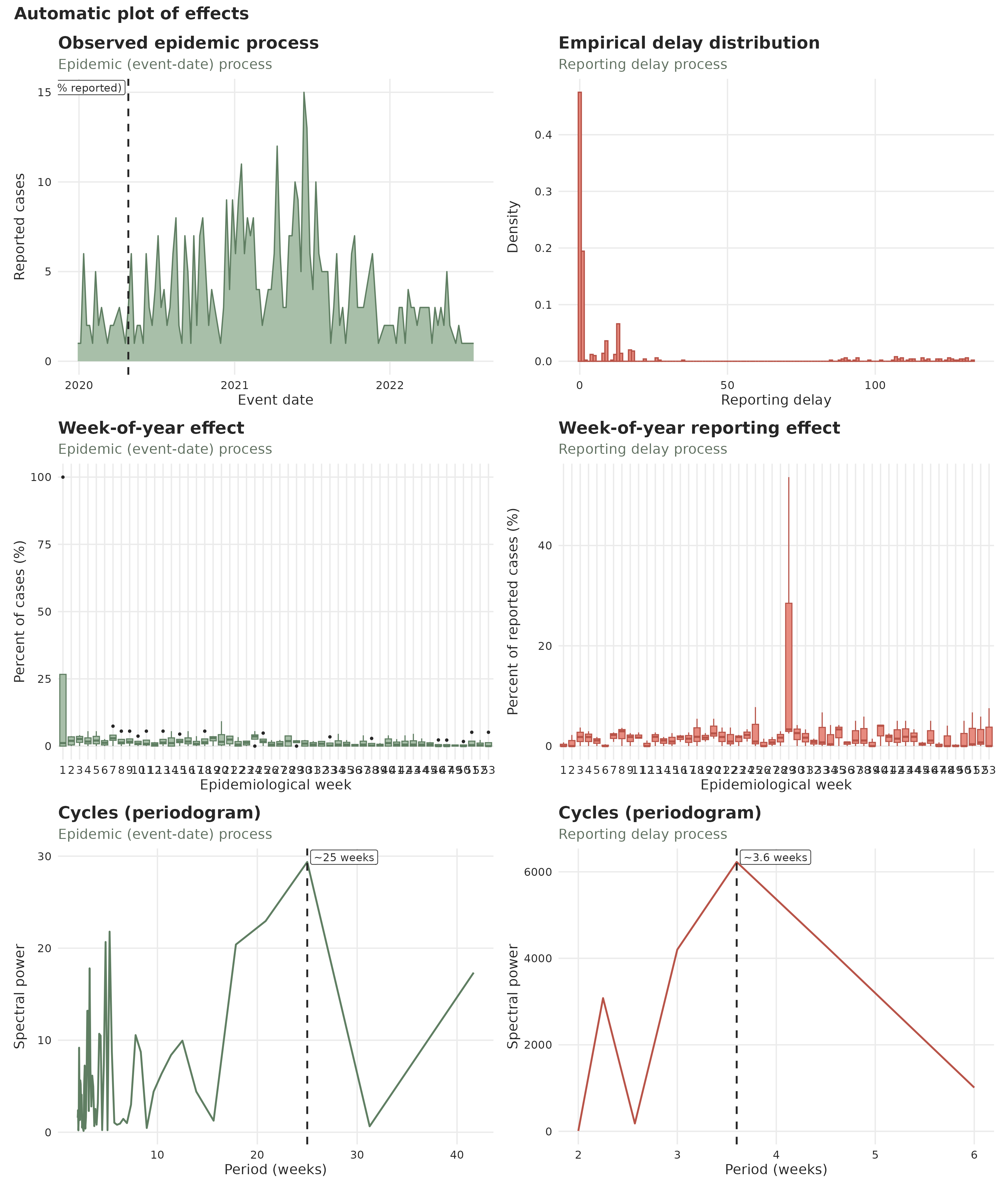

The now auto plot with weekly data

One should run again the summary() and diagnose() in the aggregated to draw conclusions from this data. For this tutorial, however it will suffice to see that the sparcity has reduced to usually just 1 week with zero cases before having cases again:

zero_run_summary(hai_bucaramanga)
#> ── Summary of a <tbl_now> ──────────────────────────────────────────────────────────────────────────────────────────────────────────────────────────────────────
#> 3 rows in 1 component; strata: "Female" and "Male".
#> 
#> zero_run
#>   n = runs of consecutive zero dates; total = zero dates in those runs
#>   quantity   stratum     n total  mean    sd   min   q25   q50   q75   q90   max
#>   <chr>      <chr>   <int> <dbl> <dbl> <dbl> <dbl> <dbl> <dbl> <dbl> <dbl> <dbl>
#> 1 event_date all         9    12  1.33 0.707     1     1     1     1     3     3
#> 2 event_date Female     28    45  1.61 0.956     1     1     1     2     3     5
#> 3 event_date Male       17    27  1.59 0.795     1     1     1     2     3     3
#> 
#> ℹ Use `dplyr::filter()` or `tibble::as_tibble()` for the full schema.

Let’s move on with the tutorial.

9. Is the reporting delay stable?

A nowcast might assume that the delay distribution is the same throughout. Here we check those assumptions:

First, we just look at the delay aggregated through time

plot_delay_drift(hai_bucaramanga)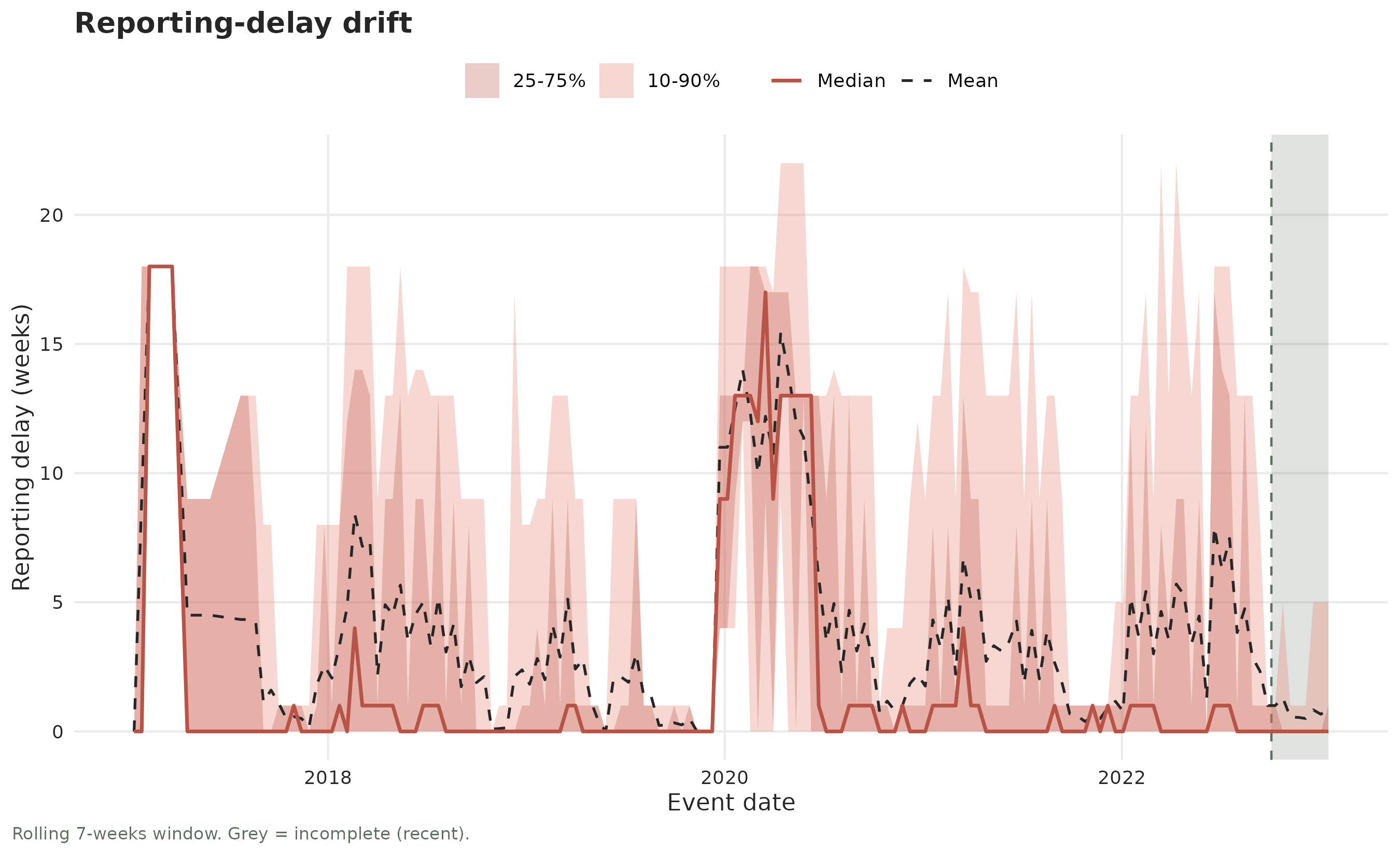

Fan chart of the reporting delay over time.

The median moves from an extremely wide distribution in 2020 to a shorter delay after 2021. We can confirm that split of two delay behaviours with the following tests:

Testing for the delay’s drift

The diagnose_drift() function runs an autocorrelation-robust Mann-Kendall test for a monotonic trend in the delay:

diagnose_drift(hai_bucaramanga)
#> # A tibble: 2 × 9
#>   strata stat       n     tau sens_slope statistic p_value method    drift
#>   <chr>  <chr>  <int>   <dbl>      <dbl>     <dbl>   <dbl> <chr>     <lgl>
#> 1 all    median    17 -0.272          -1    -3.05  0.00225 hamed-rao TRUE 
#> 2 all    spread    17 -0.0735          0    -0.503 0.615   hamed-rao FALSE

Here the median shows a reduction (sens_slope of -1) which is consistent with the plot. The -1 can be interpreted as the decrease in the median per unit of time. In this case, the median delay reduced 1 week per week.

Is there an abrupt shift?

A trend test cannot see a steep change like a jump. The diagnose_changepoint() function uses Pettitt’s test to look for exactly that.

diagnose_changepoint(hai_bucaramanga)
#> # A tibble: 2 × 10
#>   strata stat       n changepoint statistic p_value before after shift changepoint_detected
#>   <chr>  <chr>  <int> <date>          <dbl>   <dbl>  <dbl> <dbl> <dbl> <lgl>               
#> 1 all    median    17 2020-02-23         30   0.708   89.6 78.8  -10.8 FALSE               
#> 2 all    spread    17 2020-03-01         14   1       34.4  1.29 -33.1 FALSE

Here neither the median nor the spread have a changepoint. The change was a drift in the trend as we saw in the plot and not an abrupt shift. You can see the section on delay changes of the Diagnosing a tbl_now article for more information.

10. Are there any reporting batches?

A reporting batch consists on several reports that were all held for any reason by the reporter (e.g. a laboratory) and then reported all together as a group so that there is a giant signal in the reporting process. To see them we can start by plotting against the reporting axis:

plot_reporting_process(hai_bucaramanga)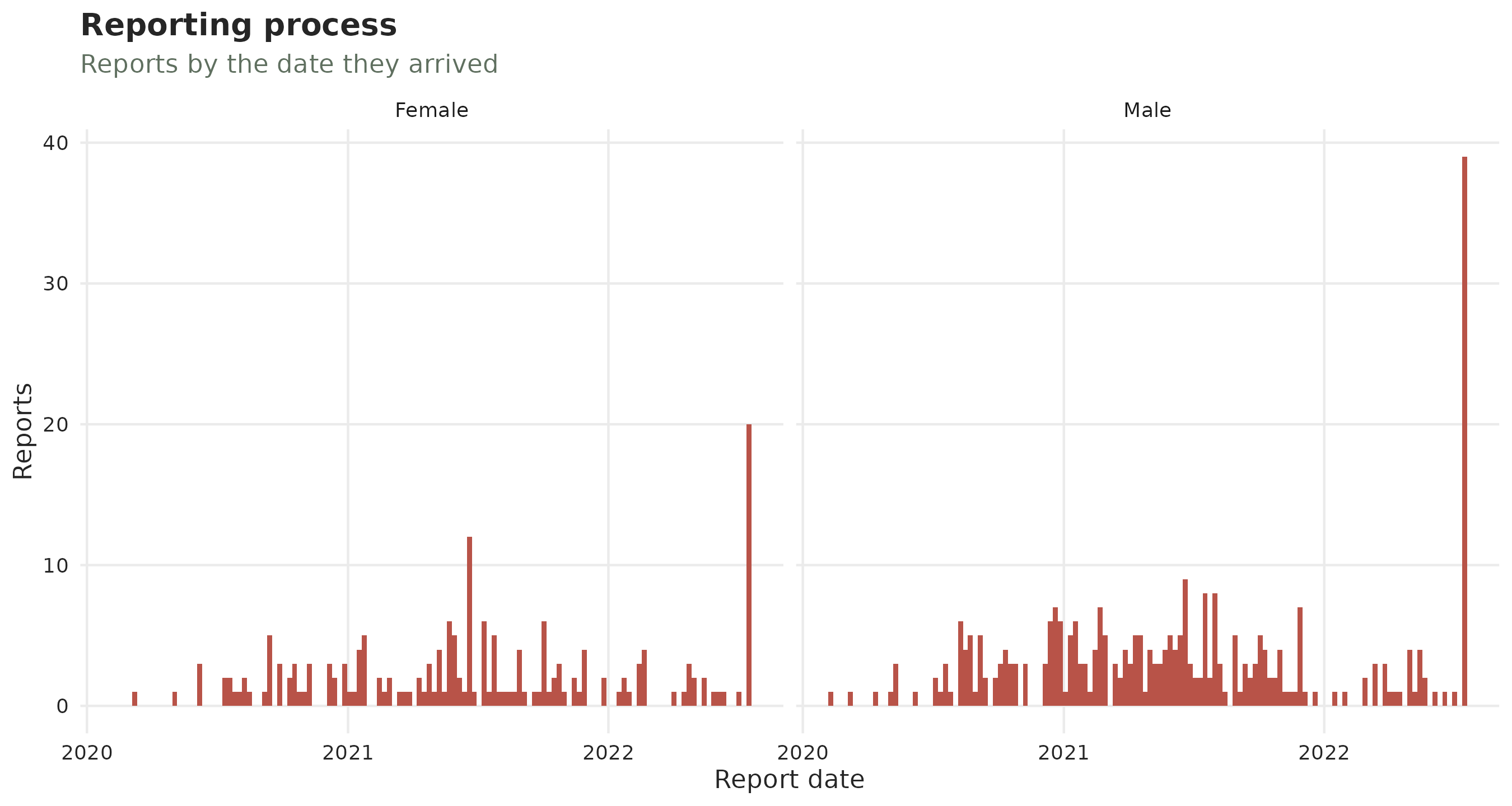

We can see that there were several reports that dropped near the end of 2022. That is our censoring. However if we didn’t know better (i.e. if we ignored that we censored it) we would analyze those reports to try to explain whether they are batches.

The reporting hexamap allows us to visualize the date of the report at the same time as the day of the event and the corresponding delay

plot_reporting_hexamap(hai_bucaramanga)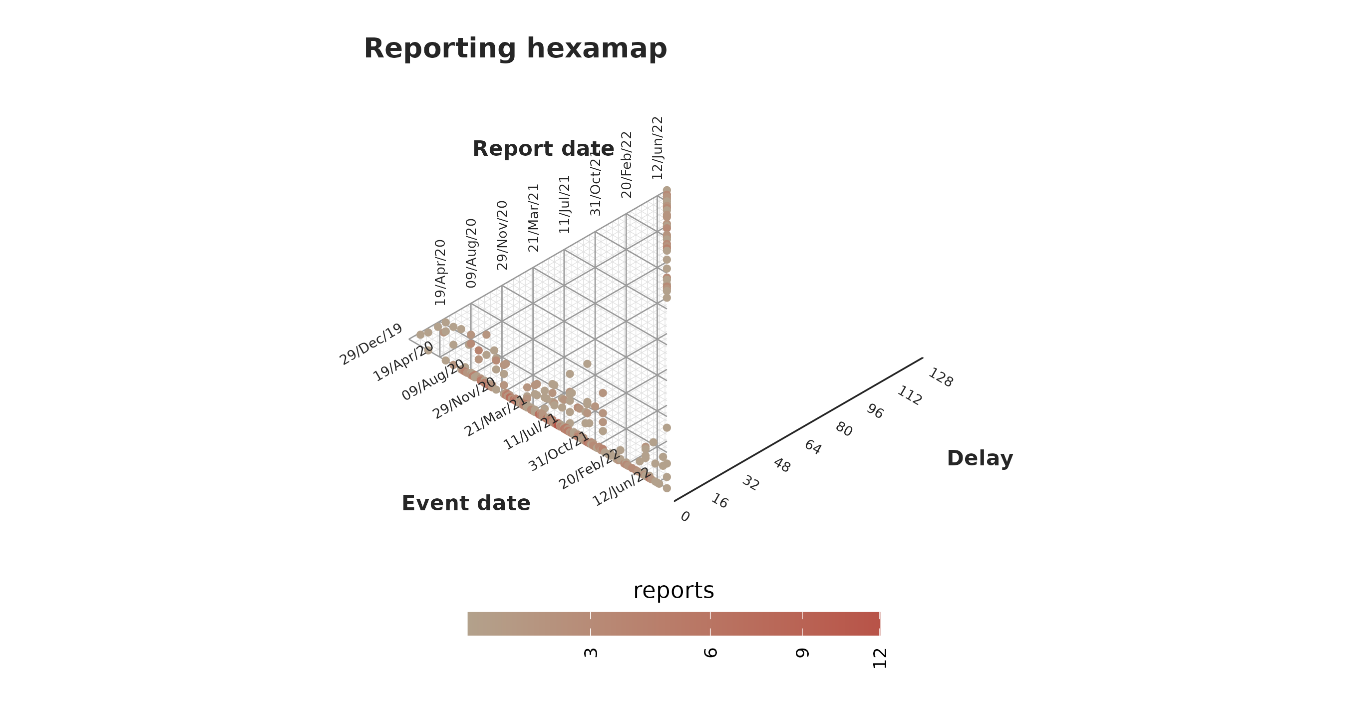

The batch at 2022-07-17 was actually introduced by us by censoring all the cases at that date in section 3.

Here lies a figure with 3 axis. We can see for example our censoring at 2022-07-17 as the collection of points in the same axis. Values shared by the same report axis with a high delay might be batches (i.e. several reported at once with some far from the event-date axis). You can see for example a point with delay around 32 weeks just before a report date of October 31st that corresponds to an event somewhere between November 2020 and Match 2021. This has a high delay and several more points were reported at that report date. We’ll come back to that.

You can also use

plot_reporting_triangle(hai_bucaramanga)

to visualize the batches; however for this specific case they are easier to visualize in the hexamap.

In this package, the diagnose_batches() function helps identify potential dates with batches. We recommend using it with or without the strata depending on whether the context warrants the possibility that batching could differ by strata (e.g. if strata correspond to healthcare facilities maybe yes; if they correspond to gender of the patient maybe no).

Here we run it without the strata which we remove first. We’ll keep only those observations that have been identified as potential batches:

hai_bucaramanga |> 
  remove_all_strata() |> 
  diagnose_batches(drop_censored = TRUE) 
#> Warning: ! `diagnose_batches()` is experimental: results are not guaranteed and the interface may change.
#> ℹ Treat a flagged report date as a potential batch, not a confirmed one.
#> This warning is displayed once every 8 hours.
#> ℹ Ignoring 58 rows flagged by .is_censored_report: a censored date is a bound, not an arrival.
#> ── Batch screen ────────────────────────────────────────────────────────────────────────────────────────────────────────────────────────────────────────────────
#> 128 (report date, stratum) pairs; look-back 7; null "poisson"
#> ⚠ 2 batches flagged at alpha = 0.05 (BH-adjusted):
#> • 2021-06-20 [all] -- reported 21, baseline 4.5, deficit -16.5, delta 33
#> • 2021-10-03 [all] -- reported 11, baseline 4, deficit 10.2, delta -3.2

This identifies some dates that might be batches due to their high reported numbers. A second batch method is the diagnose_batches2() function. This one takes a specific date and checks whether the reports that arrived on a date came from systematically older dates. We can combine the findings from the previous run to test some of them and add evidence to which are batches:

hai_bucaramanga |> 
  remove_all_strata() |> 
  diagnose_batches2(at = ymd("2021-11-28"))
#> Warning: ! `diagnose_batches2()` is experimental: results are not guaranteed and the interface may change.
#> ℹ Treat a flagged report date as a potential batch, not a confirmed one.
#> This warning is displayed once every 8 hours.
#> ℹ Ignoring 58 rows flagged by .is_censored_report: a censored date is a bound, not an arrival.
#> # A tibble: 1 × 7
#>   stratum  n_at n_reference mean_delay_at mean_delay_reference statistic p_value
#>   <chr>   <int>       <int>         <dbl>                <dbl>     <dbl>   <dbl>
#> 1 all        11          14          11.4                 2.93      2.68   0.004

Where we further identify the date of 2021-11-28 as a potential batch with its p_value < 0.05.

11. Nowcasting

Everything from sections 1 to 10 was about deciding what to fit. Three of those findings change the call we are about to make:

The object is weekly now (section 8), so now is the week of 2022-07-17 and every delay corresponds to weeks.
The reporting delay drifts down across the series. So we’ll utilize the data starting on 2021 where the delay has settled.

hai_bucaramanga <- hai_bucaramanga |> 
  filter(year(specimen_date) > 2020)

The run_nowcast() function takes the tbl_now and an engine. An engine contains a modelling package’s nowcasting function plus every argument that it needs:

hai_fit_weekly <- hai_bucaramanga |>
  run_nowcast(engine = engine_diseasenowcasting())
#> ℹ Nowcasting with "diseasenowcasting" as of 2022-07-17.
#> ℹ Added default temporal effects: 52-period seasonality (weekly data).
#> • To use your own effects, attach them to the <tbl_now> with `tbl.now::add_temporal_effects()` + `tbl.now::compute_temporal_effects()` before calling
#>   `nowcast()`.
#> • To disable, call `nowcast(..., temporal_effects = "none")`.

The autoplot() shows the nowcast with gray columns representing what had been reported by now, and the green fan the nowcast’s prediction intervals.

autoplot(hai_fit_weekly)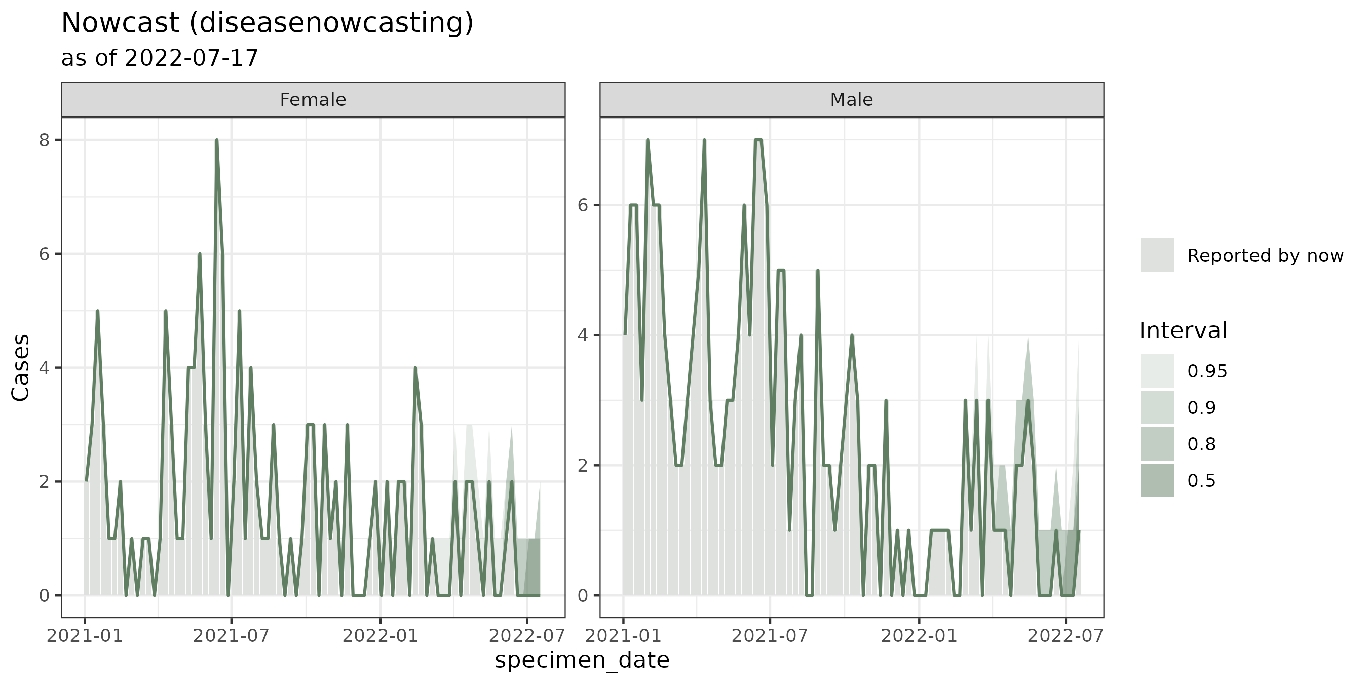

Weekly nowcast for each sex: grey columns of reported cases with a green fan of predicted cases over the final weeks.

Calling tidy() gives the nowcast as a table:

tidy(hai_fit_weekly)

#> # A tibble: 6 × 7
#>   event_date stratum estimate conf.low conf.high level engine           
#>   <date>     <chr>      <dbl>    <dbl>     <dbl> <dbl> <chr>            
#> 1 2022-07-03 Female         0        0         1  0.95 diseasenowcasting
#> 2 2022-07-03 Male           0        0         1  0.95 diseasenowcasting
#> 3 2022-07-10 Female         0        0         1  0.95 diseasenowcasting
#> 4 2022-07-10 Male           0        0         2  0.95 diseasenowcasting
#> 5 2022-07-17 Female         0        0         2  0.95 diseasenowcasting
#> # ℹ 1 more row

12. Evaluate your nowcast

One way to evaluate the nowcast is to go back in time and see what would the nowcast have produced with the information available at a previous date and contrast it with the information known by now. You can use nowcast_backtest() for that purpose: for every past date it truncates the data to the reports that were available then, refits the nowcast, and scores the result against the final observation defined by truth_axis and truth_type (reported totals by default).

To best evaluate the nowcast we need something to compare against. Hence we will fit a second model: baselinenowcast.

One can fit it with the same call just a different engine

hai_fit_baseline <- hai_bucaramanga |>
  run_nowcast(engine = engine_baselinenowcast())

Any backtest uses the same engines refitting every engine once per past date. Here we show the backtest with just 3 past dates. On a real scenario we recommend using as many as possible to draw any conclusions:

hai_backtest <- hai_bucaramanga |> 
  nowcast_backtest(
    engine_diseasenowcasting(),
    engine_baselinenowcast(),
    now_dates = c(ymd("2022-04-24"), ymd("2022-05-22"), ymd("2022-06-19")),
    seed      = 20260904
  )

The backtest is compatible with scoringutils::as_forecast_quantile() which can be used to evaluate the results:

library(scoringutils)

hai_backtest |> 
  as_forecast_quantile() |> 
  score() |> 
  summarise_scores()
#>                model        wis overprediction underprediction  dispersion        bias interval_coverage_50 interval_coverage_90  ae_median
#>               <char>      <num>          <num>           <num>       <num>       <num>                <num>                <num>      <num>
#> 1: diseasenowcasting 0.03721747   0.0002536783      0.02891933 0.008044457 -0.03732877            0.9589041            0.9817352 0.04794521
#> 2:   baselinenowcast 0.04543506   0.0012683917      0.03500761 0.009159056 -0.03470320            0.9566210            0.9726027 0.05707763

In this scenario, diseasenowcasting scores better on both accuracy measures and both methods cover far more than the nominal 90. We caution however that we cannot conclude anything from just 3 data points and in a real scenario one should use more.

Date-level indicators for the wis, ae_median and coverage can be obtained with tidy:

tidy(hai_backtest)

tidy(hai_backtest) |> arrange(event_date) |> tail()
#> # A tibble: 6 × 13
#>   method            now        event_date stratum observed estimate conf.low conf.high level    wis ae_median coverage_50 coverage_90
#>   <chr>             <date>     <date>     <chr>      <dbl>    <dbl>    <dbl>     <dbl> <dbl>  <dbl>     <dbl> <lgl>       <lgl>      
#> 1 diseasenowcasting 2022-06-19 2022-06-12 Female         2        1        1         3  0.95 0.222          1 TRUE        TRUE       
#> 2 diseasenowcasting 2022-06-19 2022-06-12 Male           0        0        0         3  0.95 0.117          0 TRUE        TRUE       
#> 3 baselinenowcast   2022-06-19 2022-06-19 Female         0        0        0         2  0.95 0.0556         0 TRUE        TRUE       
#> 4 baselinenowcast   2022-06-19 2022-06-19 Male           1        1        1         5  0.95 0.156          0 TRUE        TRUE       
#> 5 diseasenowcasting 2022-06-19 2022-06-19 Female         0        0        0         4  0.95 0.156          0 TRUE        TRUE       
#> # ℹ 1 more row

13. Ensemble nowcast

An ensemble is a weighted average between models. It leverages the fact that no model is perfect hence combining the predictions of each might lead to a more robust nowcast. You can think of an ensemble as an average of the models.

To create an ensemble model one needs to pass the model specifications as well as the backtest:

hai_ensemble <- nowcast_ensemble(
  hai_fit_weekly,
  hai_fit_baseline,
  weights  = "inverse_score",
  backtest = hai_backtest
)

The same tidy() and autoplot() functions can be used here:

autoplot(hai_ensemble)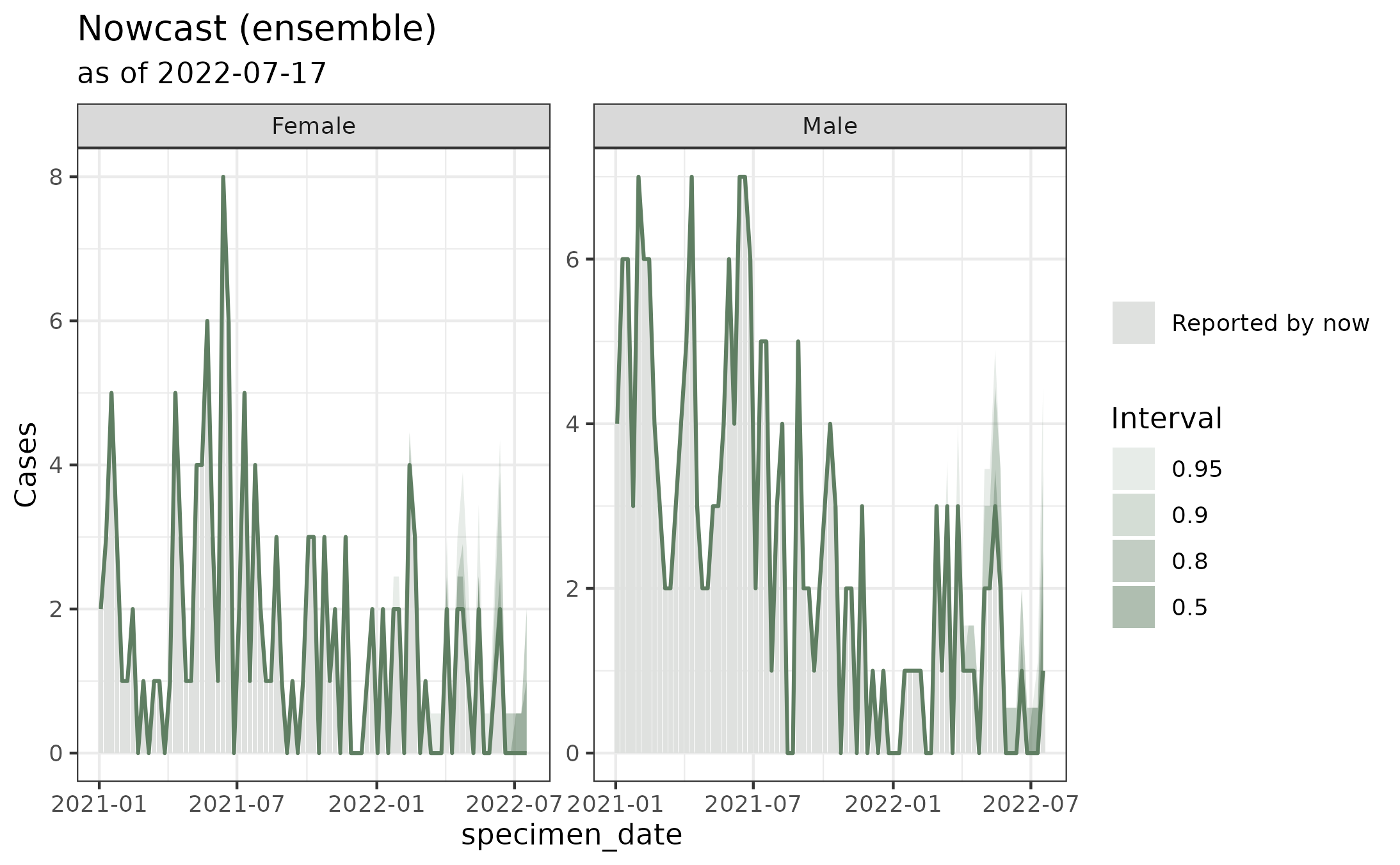

One can fit ensembles with more than two models and different model specifications. Check out the article on ensemble nowcasting for more information.

Summary

In this example we showed:

How to create a tbl_now() object.
How to diagnose() and summarise with summary() as well as visualize with autoplot() a tbl_now().
How to add temporal_effects() to the object which can be displayed in the plots.
How to aggregate the time units with aggregate_time_units() to pass from days to weeks.
How to identify drifts and batches with plot_delay_drift(), diagnose_drift() and diagnose_changepoint(). 6. How to identify potential batches with plot_reporting_hexamap() in conjunction with diagnose_batches() (and diagnose_batches2()).
How to perform a nowcast by setting an engine() and running with run_nowcast().
How to clean with tidy() and autoplot() a nowcast.
How to backtest a nowcast with nowcast_backtest() and create an ensemble with nowcast_ensemble().

If you have any questions or comments regarding the contents of this article please open an issue on Github.

Learning more

A tutorial on real life surveillance data. Takes you from cleaning to diagnosing errors in the data to nowcasting: https://rodrigozepeda.github.io/tbl.now/articles/example.html
The second part of the tutorial with a revision process: the optional third date, where a reported case is later confirmed, retracted or left pending: https://rodrigozepeda.github.io/tbl.now/articles/example_revisions.html
The Get started vignette: the whole workflow, from a raw line list to a scored nowcast, in five minutes: https://rodrigozepeda.github.io/tbl.now/articles/tbl.now.html.
More on the tbl_now object: every attribute, the three data types, the revision process, temporal effects and the dplyr methods: https://rodrigozepeda.github.io/tbl.now/articles/more-on-tbl-now.html
More thoughts on diagnosing your dataset with tbl.now https://rodrigozepeda.github.io/tbl.now/articles/diagnosing-a-tbl-now.html
Detecting reporting batches with tbl.now https://rodrigozepeda.github.io/tbl.now/articles/batches.html
How to use different nowcasting engines from tbl.now: here you can learn how it connects to the other nowcasting packages. https://rodrigozepeda.github.io/tbl.now/articles/nowcasting-models.html
How to nowcast with multiple engines, backtest and ensemble nowcasts. https://rodrigozepeda.github.io/tbl.now/articles/ensemble-nowcasting.html
Adding your own custom nowcasting model https://rodrigozepeda.github.io/tbl.now/articles/custom-nowcast-models.html
Package reference: https://rodrigozepeda.github.io/tbl.now/reference/