More on the tbl_now object

Why this vignette

This article describes in depth a tbl_now: what it records, every attribute it carries, how it goes through a dplyr pipeline, and the additional functions that come with it. If you have not met the package yet, read the Get started vignette first.

Introduction

The tbl.now extends a regular tibble() to explicitly encode epidemiological event and report dates, allowing consistent data transformation, delay computation, and integration with the diseasenowcasting and other modeling workflows.

More concretely, tbl.now was designed to:

Standardize the data inputs required by nowcasting models (including diseasenowcasting).
Preserve tidyverse compatibility so users can continue to apply familiar dplyr operations.
Diagnose reporting artifacts directly from the data (such as reporting-delay drift and change points) as well as batch (backlog) reporting.
Facilitate integration into iterative modeling workflows with different nowcasting packages (Gelman et al. 2020; Wickham et al. 2023):
Facility backtesting and ensembling of nowcasts

We begin by loading the required packages:

library(dplyr, quietly = TRUE)
library(lubridate)
library(tbl.now)

How `tbl.now` works

In an epidemiological nowcast, we typically observe at least two key dates¹:

event_date: when the underlying event occurred (e.g., symptom onset, exposure, sample collection).
report_date: when the event was recorded in the data system (e.g., lab result processed, clinical visit documented).

The nowcasting task is:

To estimate, for each past event_date, how many events (e.g. cases) have already occurred but have not yet been reported as of now. That is, the nowcast will predict how many observations will eventually be observed for each (past or present) event_date.

Visually:

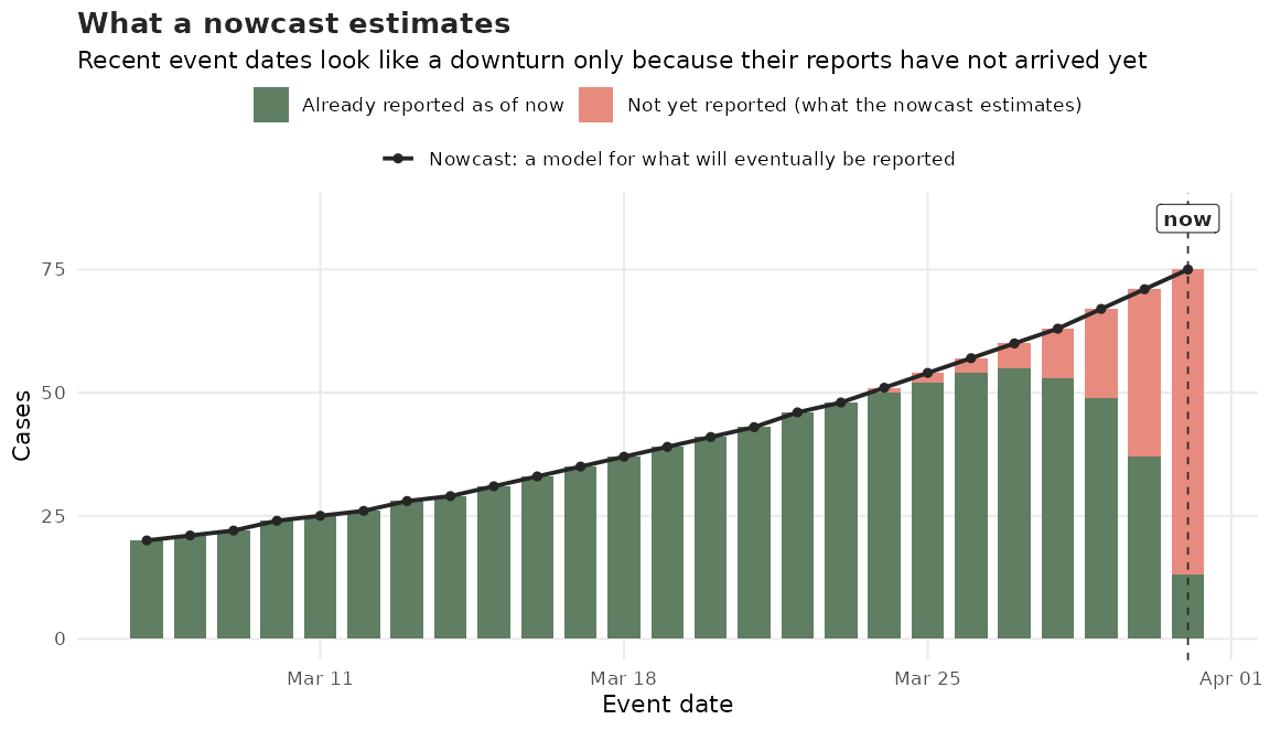
Stacked bar chart of cases by event date. Green bars show cases already reported as of now; pale red bars stacked on top show the cases not yet reported, which grow rapidly over the most recent event dates. A black line traces the total that will eventually be reported, rising steadily, while the green observed bars turn downward near now.

In the figure above, the green bars represent the number of cases (events) that have been observed until now; the pale red segments are the reports still in transit. Because completeness decays sharply over the most recent event dates, the observed counts bend downwards near the right edge even though the epidemic is still growing. The nowcast is the red line: an estimate of the height each bar will eventually reach.

A tbl.now object is a specialized tibble() that:

Identifies the event_date and report_date columns.
Stores these as attributes() to enable consistent processing.
Automatically computes auxiliary fields such as delay, numerical indices, and frequency units.
Ensures the dataset is correctly formatted for multiple frameworks including diseasenowcasting, epidist, epinow, NobBS, and more (see list_nowcast_methods()).

Example: A simple `tbl.now`

Consider the following dataset:

symptom_onset	medical_visit	n
2023-12-25	2023-12-26	10
2023-12-26	2023-12-26	2
2023-12-25	2023-12-27	5
2023-12-26	2023-12-27	11

Where:

symptom_onset is the event_date.
medical_visit is the report_date.
n is the number of reported cases for each event–report combination.

We can convert this into a tbl_now() by first creating a data.frame and then using the tbl_now() function:

#Create a data.frame
df <- data.frame(
  symptom_onset = c(ymd("2023/12/25"), ymd("2023/12/26"), 
                    ymd("2023/12/25"), ymd("2023/12/26")),
  medical_visit = c(ymd("2023/12/26"), ymd("2023/12/26"), 
                    ymd("2023/12/27"), ymd("2023/12/27")),
  n = c(10, 2, 5, 11)
)

#Convert to tbl.now
df |>
  tbl_now(event_date = symptom_onset, report_date = medical_visit, case_count = n)
#> ℹ Identified data as <count-incidence> with counts in column "n".
#> # A tibble:  4 × 6
#> # Data type: "count-incidence"
#> # Frequency: Event: `days` | Report: `days`
#>   symptom_onset medical_visit       n .event_num .report_num .delay
#>   <date>        <date>          <dbl>      <dbl>       <dbl>  <dbl>
#>   [event_date]  [report_date] [cases]      [...]       [...]  [...]
#> 1 2023-12-25    2023-12-26         10          0           1      1
#> 2 2023-12-26    2023-12-26          2          1           1      0
#> 3 2023-12-25    2023-12-27          5          0           2      2
#> 4 2023-12-26    2023-12-27         11          1           2      1
#> # ────────────────────────────────────────────────────────────────────────────────
#> # Now: 2023-12-27 | Event date: "symptom_onset" | Report date: "medical_visit"
#> # ────────────────────────────────────────────────────────────────────────────────

This performs several operations automatically:

Detects the data type (count-incidence in this example). See below for all the data types available.
Infers the frequency units of event and report dates (daily).
Tags the correct columns as event_date, report_date, and case_count.
Computes .event_num, .report_num, and .delay columns the numerical versions (indexed at 0) of event, report and .delay = report_date - event_date columns.
Identifies the appropriate now date (the most recent report date).

The remaining sections describe these features and the broader tbl.now toolkit.

Attributes of a tbl_now()

A tbl_now() stores information about its structure using object attributes, ensuring consistent behavior across dplyr transformations. The primary attributes are:

	Argument	What it records
	`event_date`	The column storing event dates; i.e. when the epidemiological phenomenon of interest happened (symptom onset, hospitalisation, death, …). Required.
	`report_date`	The column storing report dates; i.e. when that event became known to the surveillance system. Required, unless it is reconstructed from `delay`.
	`revision_date`	An optional third date indicating when the report was resolved (see `revision_type`). Optional.
	`revision_type`, `revision_levels`	What the revision date resolved to. Only `confirmed`, `retracted`, `pending` or `NA` are ever stored; set `revision_levels` as a named dictionary mapping the data’s labels into those four ( e.g. `c(positive = “confirmed”)`). Optional.
	`now`	The date the nowcast is anchored to — “today” from the model’s point of view. Optional; defaults to the latest date.
	`strata`	Columns you want a separate nowcast for (e.g. gender, region). Optional.
	`covariates`	Columns that inform the nowcast but that you do not want it broken down by (e.g. temperature or precipitation). Optional.
	`case_count`	The column holding the counts when the data is given as aggregated (rather than line-list). Optional.
	`data_type`	Whether the data represents a `linelist` (each row is a case), `count-incidence`(each row is a collection of cases per event-report date) or `count-cumulative`(each row is the cummulative number cases for that event accumulating in the report axis). Optional; inferred by default.
	`event_units`, `report_units`, `revision_units`	The time grid each date lives on: `days`, `weeks`, `months`, `years` or `numeric`. Optional; inferred (`“auto”`) by default.
	`is_censored_report`,`is_censored_revision`	Flags dates from either the report or the revision axis that are only an upper bound, i.e. the true report happened before the date given in the database. Optional.
	`t_effects`	Columns holding temporal effects (day of week, holidays, …) that some models can use. Optional.

On top of these, a tbl_now keeps the generated columns it computes for you: .event_num, .report_num and .delay, plus .revision_num and .revision_delay when there is a revision date. They are protected: removing or renaming one demotes the object back to an ordinary tibble, because the rest of the package can no longer trust it.

You can access any attribute using the corresponding getter, e.g. get_event_date() or get_strata().

Below we provide more information on some of the attributes.

Data types

A tbl_now() can represent one of three data structures:

Linelist: Each row corresponds to a single reported observation.

Linelist data
patient	event_date	report_date
1	2020-09-12	2020-09-12
2	2020-09-12	2020-09-12
3	2020-09-12	2020-09-13
4	2020-09-13	2020-09-13
5	2020-09-13	2020-09-13
6	2020-09-13	2020-09-13

Count-incidence: Each row summarizes how many events with a given event_date were reported exactly on that report_date.

Count-incidence data
n	event_date	report_date
7	2020-09-12	2020-09-12
1	2020-09-12	2020-09-13
9	2020-09-12	2020-09-14
5	2020-09-13	2020-09-13
0	2020-09-13	2020-09-14
2	2020-09-13	2020-09-15

Count-cumulative Each row summarizes how many events with a given event_date had been reported up to and including that report_date. The distinction is crucial for nowcasting models that operate either on daily increments or cumulative totals.

Count-cumulative data
n	event_date	report_date
1	2020-09-12	2020-09-12
5	2020-09-12	2020-09-13
8	2020-09-12	2020-09-14
2	2020-09-13	2020-09-13
2	2020-09-13	2020-09-14
4	2020-09-13	2020-09-15

The to_count() function allows you to convert between different data-types as we see below:

Converting Between Data Types

The to_count() function supports structured transformations. Here we start with linelist data as an example:

#The original data.frame has one row per patient
df_linelist <- data.frame(
  patient     = 1:6,
  event_date  = c(rep(ymd("2020/09/12"), 3), rep(ymd("2020/09/13"), 3)),
  report_date = c(rep(ymd("2020/09/12"), 2), rep(ymd("2020/09/13"), 4))
)

#We can convert it to a tbl.now
df_linelist <- df_linelist |> 
  tbl_now(event_date = event_date, report_date = report_date, 
          data_type = "linelist")

#This is what it looks like
df_linelist
#> # A tibble:  6 × 6
#> # Data type: "linelist"
#> # Frequency: Event: `days` | Report: `days`
#>   patient event_date   report_date   .event_num .report_num .delay
#>     <int> <date>       <date>             <dbl>       <dbl>  <dbl>
#>     [...] [event_date] [report_date]      [...]       [...]  [...]
#> 1       1 2020-09-12   2020-09-12             0           0      0
#> 2       2 2020-09-12   2020-09-12             0           0      0
#> 3       3 2020-09-12   2020-09-13             0           1      1
#> 4       4 2020-09-13   2020-09-13             1           1      0
#> 5       5 2020-09-13   2020-09-13             1           1      0
#> 6       6 2020-09-13   2020-09-13             1           1      0
#> # ────────────────────────────────────────────────────────────────────────────────
#> # Now: 2020-09-13 | Event date: "event_date" | Report date: "report_date"
#> # ────────────────────────────────────────────────────────────────────────────────

Linelist → Count-Incidence: Aggregates by event–report date, counting only cases reported on that date.

df_linelist |>
  to_count(to = "count-incidence")
#> # A tibble:  3 × 6
#> # Data type: "count-incidence"
#> # Frequency: Event: `days` | Report: `days`
#>   event_date   report_date   .event_num .report_num       n .delay
#>   <date>       <date>             <dbl>       <dbl>   <int>  <dbl>
#>   [event_date] [report_date]      [...]       [...] [cases]  [...]
#> 1 2020-09-12   2020-09-12             0           0       2      0
#> 2 2020-09-12   2020-09-13             0           1       1      1
#> 3 2020-09-13   2020-09-13             1           1       3      0
#> # ────────────────────────────────────────────────────────────────────────────────
#> # Now: 2020-09-13 | Event date: "event_date" | Report date: "report_date"
#> # ────────────────────────────────────────────────────────────────────────────────

Linelist → Count-Cumulative: Aggregates by event–report date, producing cumulative counts up to each report date.

df_linelist |>
  to_count(to = "count-cumulative")
#> # A tibble:  3 × 6
#> # Data type: "count-cumulative"
#> # Frequency: Event: `days` | Report: `days`
#>   event_date   report_date   .event_num .report_num       n .delay
#>   <date>       <date>             <dbl>       <dbl>   <int>  <dbl>
#>   [event_date] [report_date]      [...]       [...] [cases]  [...]
#> 1 2020-09-12   2020-09-12             0           0       2      0
#> 2 2020-09-12   2020-09-13             0           1       3      1
#> 3 2020-09-13   2020-09-13             1           1       3      0
#> # ────────────────────────────────────────────────────────────────────────────────
#> # Now: 2020-09-13 | Event date: "event_date" | Report date: "report_date"
#> # ────────────────────────────────────────────────────────────────────────────────

Note In the previous example the n counts 3 as it is aggregating the 1 observed at report_date = 2020-09-13 and the 2 observed at report_date = 2020-09-12. This is the difference between the count-incidence that specifies the ones observed exactly on that date and the count-cumulative that specifies the ones observed up until and including that date.

Count-Incidence → Count-Cumulative: Computes cumulative sums for each event date across report dates.

df_count_inc <- df_linelist |>
  to_count(to = "count-incidence")

#This is count incidence:
df_count_inc
#> # A tibble:  3 × 6
#> # Data type: "count-incidence"
#> # Frequency: Event: `days` | Report: `days`
#>   event_date   report_date   .event_num .report_num       n .delay
#>   <date>       <date>             <dbl>       <dbl>   <int>  <dbl>
#>   [event_date] [report_date]      [...]       [...] [cases]  [...]
#> 1 2020-09-12   2020-09-12             0           0       2      0
#> 2 2020-09-12   2020-09-13             0           1       1      1
#> 3 2020-09-13   2020-09-13             1           1       3      0
#> # ────────────────────────────────────────────────────────────────────────────────
#> # Now: 2020-09-13 | Event date: "event_date" | Report date: "report_date"
#> # ────────────────────────────────────────────────────────────────────────────────

#Turns to count cumulative:
df_count_inc |>
  to_count(to = "count-cumulative")
#> # A tibble:  3 × 6
#> # Data type: "count-cumulative"
#> # Frequency: Event: `days` | Report: `days`
#>   event_date   report_date   .event_num .report_num       n .delay
#>   <date>       <date>             <dbl>       <dbl>   <int>  <dbl>
#>   [event_date] [report_date]      [...]       [...] [cases]  [...]
#> 1 2020-09-12   2020-09-12             0           0       2      0
#> 2 2020-09-12   2020-09-13             0           1       3      1
#> 3 2020-09-13   2020-09-13             1           1       3      0
#> # ────────────────────────────────────────────────────────────────────────────────
#> # Now: 2020-09-13 | Event date: "event_date" | Report date: "report_date"
#> # ────────────────────────────────────────────────────────────────────────────────

Aggregation within the same type: The to_count() may also be used to re-aggregate datasets that contain duplicate event–report pairs. This is useful when raw surveillance feeds contain repeated entries such as in this case:

tbl_example <- data.frame(
  n = c(8, 11, 0, 1, 1, 5, 2, 4, 1, 10, 9, 11, 3, 1),
  sex = c(rep("M", 3), rep("F", 4), rep("M", 2), rep("F", 5)),
  event_date = c(
    rep(ymd("2020/09/12"), 3),
    rep(ymd("2020/09/12"), 4),
    rep(ymd("2020/09/13"), 2),
    rep(ymd("2020/09/13"), 5)
  ),
  report_date = c(
    ymd("2020/09/12"), ymd("2020/09/13"), ymd("2020/09/14"),
    ymd("2020/09/12"), ymd("2020/09/13"), ymd("2020/09/14"),
    ymd("2020/09/15"), ymd("2020/09/13"), ymd("2020/09/14"),
    ymd("2020/09/13"), ymd("2020/09/14"),
    ymd("2020/09/15"), ymd("2020/09/16"), ymd("2020/09/17")
  )) |>
  tbl_now(
    event_date = event_date, report_date = report_date,
    data_type = "count-incidence", case_count = n, verbose = FALSE,
    warn_non_uniqueness = FALSE
  )

tbl_example
#> # A tibble:  14 × 7
#> # Data type: "count-incidence"
#> # Frequency: Event: `days` | Report: `days`
#>          n sex   event_date   report_date   .event_num .report_num .delay
#>      <dbl> <chr> <date>       <date>             <dbl>       <dbl>  <dbl>
#>    [cases] [...] [event_date] [report_date]      [...]       [...]  [...]
#>  1       8 M     2020-09-12   2020-09-12             0           0      0
#>  2      11 M     2020-09-12   2020-09-13             0           1      1
#>  3       0 M     2020-09-12   2020-09-14             0           2      2
#>  4       1 F     2020-09-12   2020-09-12             0           0      0
#>  5       1 F     2020-09-12   2020-09-13             0           1      1
#>  6       5 F     2020-09-12   2020-09-14             0           2      2
#>  7       2 F     2020-09-12   2020-09-15             0           3      3
#>  8       4 M     2020-09-13   2020-09-13             1           1      0
#>  9       1 M     2020-09-13   2020-09-14             1           2      1
#> 10      10 F     2020-09-13   2020-09-13             1           1      0
#> 11       9 F     2020-09-13   2020-09-14             1           2      1
#> 12      11 F     2020-09-13   2020-09-15             1           3      2
#> 13       3 F     2020-09-13   2020-09-16             1           4      3
#> 14       1 F     2020-09-13   2020-09-17             1           5      4
#> # ────────────────────────────────────────────────────────────────────────────────
#> # Now: 2020-09-17 | Event date: "event_date" | Report date: "report_date"
#> # ────────────────────────────────────────────────────────────────────────────────

This dataset intentionally contains repeated event_date–report_date pairs for each sex. You can aggregate redundant rows with the to_count() function that collapses duplicates by summing the case_count column.

tbl_example |>
  to_count(to = "count-incidence")
#> # A tibble:  9 × 6
#> # Data type: "count-incidence"
#> # Frequency: Event: `days` | Report: `days`
#>   event_date   report_date   .event_num .report_num       n .delay
#>   <date>       <date>             <dbl>       <dbl>   <dbl>  <dbl>
#>   [event_date] [report_date]      [...]       [...] [cases]  [...]
#> 1 2020-09-12   2020-09-12             0           0       9      0
#> 2 2020-09-12   2020-09-13             0           1      12      1
#> 3 2020-09-12   2020-09-14             0           2       5      2
#> 4 2020-09-12   2020-09-15             0           3       2      3
#> 5 2020-09-13   2020-09-13             1           1      14      0
#> 6 2020-09-13   2020-09-14             1           2      10      1
#> 7 2020-09-13   2020-09-15             1           3      11      2
#> 8 2020-09-13   2020-09-16             1           4       3      3
#> 9 2020-09-13   2020-09-17             1           5       1      4
#> # ────────────────────────────────────────────────────────────────────────────────
#> # Now: 2020-09-17 | Event date: "event_date" | Report date: "report_date"
#> # ────────────────────────────────────────────────────────────────────────────────

The function ensures that:

Rows are grouped by event_date, report_date, and any strata, and is_censored_report.
The case_count column is summed within each group.
Attributes are preserved so the resulting object remains a valid tbl_now.

Changing the time unit

to_count() changes if there is a count and what the count column is; it does not change how long a period is. Sometimes, surveillance data is too sparse to nowcast and the usual fix is to work in weeks. The aggregate_time_units() function moves every date onto a coarser time-grid. For example passing from daily data:

daily <- data.frame(
  onset    = ymd("2024/01/01") + c(0, 1, 3, 8, 9, 15),
  reported = ymd("2024/01/01") + c(2, 2, 5, 9, 12, 16),
  sex      = c("F", "M", "F", "M", "F", "M")
) |>
  tbl_now(
    event_date = onset, report_date = reported, strata = sex,
    data_type = "linelist", units = "days", verbose = FALSE
  )

daily
#> # A tibble:  6 × 6
#> # Data type: "linelist"
#> # Frequency: Event: `days` | Report: `days`
#>   onset        reported      sex      .event_num .report_num .delay
#>   <date>       <date>        <chr>         <dbl>       <dbl>  <dbl>
#>   [event_date] [report_date] [strata]      [...]       [...]  [...]
#> 1 2024-01-01   2024-01-03    F                 0           2      2
#> 2 2024-01-02   2024-01-03    M                 1           2      1
#> 3 2024-01-04   2024-01-06    F                 3           5      2
#> 4 2024-01-09   2024-01-10    M                 8           9      1
#> 5 2024-01-10   2024-01-13    F                 9          12      3
#> 6 2024-01-16   2024-01-17    M                15          16      1
#> # ────────────────────────────────────────────────────────────────────────────────
#> # Now: 2024-01-17 | Event date: "onset" | Report date: "reported"
#> # Strata: "sex"
#> # ────────────────────────────────────────────────────────────────────────────────

to weekly:

weekly <- daily |> 
  aggregate_time_units(to = "weeks", verbose = FALSE)

weekly
#> # A tibble:  6 × 6
#> # Data type: "linelist"
#> # Frequency: Event: `weeks` | Report: `weeks`
#>   onset        reported      sex      .event_num .report_num .delay
#>   <date>       <date>        <chr>         <dbl>       <dbl>  <dbl>
#>   [event_date] [report_date] [strata]      [...]       [...]  [...]
#> 1 2023-12-31   2023-12-31    F                 0           0      0
#> 2 2023-12-31   2023-12-31    M                 0           0      0
#> 3 2023-12-31   2023-12-31    F                 0           0      0
#> 4 2024-01-07   2024-01-07    M                 1           1      0
#> 5 2024-01-07   2024-01-07    F                 1           1      0
#> 6 2024-01-14   2024-01-14    M                 2           2      0
#> # ────────────────────────────────────────────────────────────────────────────────
#> # Now: 2024-01-14 | Event date: "onset" | Report date: "reported"
#> # Strata: "sex"
#> # ────────────────────────────────────────────────────────────────────────────────

Censoring the dates that are not really dates

Surveillance data arrives with missing report dates or stand-ins such as 2222-02-22 for “never reported”. Deleting those rows throws away real cases; believing them makes the nowcast think reporting is far slower than it is. The censoring keep the case and record its delay as an upper bound:

messy <- data.frame(
  onset    = ymd("2020/01/01") + 0:3,
  reported = ymd(c("2020/01/03", NA, "2222/02/22", "2020/01/06"))
  ) |>
  tbl_now(
    event_date = onset, report_date = reported, data_type = "linelist",
    units = "days", now = ymd("2020/01/10"), verbose = FALSE
  ) 

#Here we use a condition to tell what reports should be upper bounded
fixed <- messy |>
  censor_reports(
    is.na(reported) | reported > ymd("2100/01/01"), 
    to_report = ymd("2020/01/10"), verbose = FALSE
  ) 

fixed
#> # A tibble:  4 × 6
#> # Data type: "linelist"
#> # Frequency: Event: `days` | Report: `days`
#>   onset        reported      .is_censored_report  .event_num .report_num .delay
#>   <date>       <date>        <lgl>                     <dbl>       <dbl>  <dbl>
#>   [event_date] [report_date] [is_censored_report]      [...]       [...]  [...]
#> 1 2020-01-01   2020-01-03    FALSE                         0           2      2
#> 2 2020-01-02   2020-01-10    TRUE                          1           9      8
#> 3 2020-01-03   2020-01-10    TRUE                          2           9      7
#> 4 2020-01-04   2020-01-06    FALSE                         3           5      2
#> # ────────────────────────────────────────────────────────────────────────────────
#> # Now: 2020-01-10 | Event date: "onset" | Report date: "reported"
#> # left-censored indicator: ".is_censored_report"
#> # ────────────────────────────────────────────────────────────────────────────────

The main idea is that reports are always upper bounded (if you are seeing a report today then the most recent date it could have arrived is today!). Some nowcasting models work with these censored frameworks.

Temporal effects

Oftentimes, temporal covariates improve nowcasting performance by helping to adjust systematic changes within the calendar cycle (e.g., day-of-week effects, seasonal effects, or other reporting artefacts). The temporal_effects() function creates a specification (recipe) of the features to compute:

library(almanac)

t_eff <- temporal_effects(
  day_of_week  = TRUE,
  week_of_year = TRUE,
  holidays     = cal_us_federal()
)

t_eff
#> ── Temporal Effects ────────────────────────────────────────────────────────────
#> The following effects are in place:
#> • "day_of_week"
#> • "week_of_year"
#> • "holidays":
#>     New Year's Day, US Martin Luther King Jr. Day, US Presidents' Day, US Memorial Day, US Juneteenth, US Independence Day, US Labor Day, US Indigenous Peoples' Day, US Veterans Day, US Thanksgiving, and Christmas

Note that the holidays calendar is an rcalendar object from the almanac package.

How do they work?

Temporal effects in tbl.now follow a lazy evaluation pattern:

Add with add_temporal_effects() (or via the t_effects argument of tbl_now()). This records what should be computed but adds no columns yet.
Materialise the columns with compute_temporal_effects() when you are ready to use them in a model.

data("denguedat")

# Step 1 — create the tbl_now and attach the spec (no columns added yet)
df_now <- denguedat |>
  tbl_now(
    event_date = onset_week, report_date = report_week,
    verbose = FALSE, strata = gender
  )

df_now <- df_now |>
  add_temporal_effects(t_eff)

# The footer shows "T. effects (lazy): ..." — spec is recorded but not computed
df_now
#> # A tibble:  52,987 × 6
#> # Data type: "linelist"
#> # Frequency: Event: `weeks` | Report: `weeks`
#>    onset_week   report_week   gender   .event_num .report_num .delay
#>    <date>       <date>        <chr>         <dbl>       <dbl>  <dbl>
#>    [event_date] [report_date] [strata]      [...]       [...]  [...]
#>  1 1990-01-01   1990-01-01    Male              0           0      0
#>  2 1990-01-01   1990-01-01    Female            0           0      0
#>  3 1990-01-01   1990-01-01    Female            0           0      0
#>  4 1990-01-01   1990-01-08    Female            0           1      1
#>  5 1990-01-01   1990-01-08    Male              0           1      1
#>  6 1990-01-01   1990-01-15    Female            0           2      2
#>  7 1990-01-01   1990-01-15    Female            0           2      2
#>  8 1990-01-01   1990-01-15    Female            0           2      2
#>  9 1990-01-01   1990-01-22    Female            0           3      3
#> 10 1990-01-01   1990-01-08    Female            0           1      1
#> # ────────────────────────────────────────────────────────────────────────────────
#> # Now: 2010-12-20 | Event date: "onset_week" | Report date: "report_week"
#> # Strata: "gender"
#> # T. effects (lazy): [event_date] day_of_week, week_of_year, holidays
#> # ────────────────────────────────────────────────────────────────────────────────
#> # ℹ 52,977 more rows

The footer now shows the spec with (lazy) to signal that the columns have not been computed yet. No new columns appear in the tibble at this point. When we compute, they appear (scroll to the right):

# Step 2 — materialise the columns when needed
df_computed <- compute_temporal_effects(df_now)

# Columns are now present and annotated [t_effect]
df_computed
#> # A tibble:  52,987 × 9
#> # Data type: "linelist"
#> # Frequency: Event: `weeks` | Report: `weeks`
#>    onset_week   report_week   gender   .event_num .report_num .delay
#>    <date>       <date>        <chr>         <dbl>       <dbl>  <dbl>
#>    [event_date] [report_date] [strata]      [...]       [...]  [...]
#>  1 1990-01-01   1990-01-01    Male              0           0      0
#>  2 1990-01-01   1990-01-01    Female            0           0      0
#>  3 1990-01-01   1990-01-01    Female            0           0      0
#>  4 1990-01-01   1990-01-08    Female            0           1      1
#>  5 1990-01-01   1990-01-08    Male              0           1      1
#>  6 1990-01-01   1990-01-15    Female            0           2      2
#>  7 1990-01-01   1990-01-15    Female            0           2      2
#>  8 1990-01-01   1990-01-15    Female            0           2      2
#>  9 1990-01-01   1990-01-22    Female            0           3      3
#> 10 1990-01-01   1990-01-08    Female            0           1      1
#> # ────────────────────────────────────────────────────────────────────────────────
#> # Now: 2010-12-20 | Event date: "onset_week" | Report date: "report_week"
#> # Strata: "gender"
#> # T. effects: [event_date] day_of_week, week_of_year, holidays
#> # T. effect cols: ".event_day_of_week", ".event_week_of_year", and
#> # ".event_holiday"
#> # ────────────────────────────────────────────────────────────────────────────────
#> # ℹ 52,977 more rows
#> # ℹ 3 more variables: .event_day_of_week <fct>, .event_week_of_year <fct>,
#> #   .event_holiday <dbl>

After compute_temporal_effects():

The effect columns (.event_day_of_week, .event_week_of_year, .event_holiday) are added.
The function get_temporal_effect_cols() lists the column names while
The original call remains accessible via get_temporal_effects(), so you always know which effects were requested even after further dplyr operations.

get_temporal_effects(df_computed)     # The spec (list of configs)
#> [[1]]
#> [[1]]$t_effects
#> ── Temporal Effects ────────────────────────────────────────────────────────────
#> The following effects are in place:
#> • "day_of_week"
#> • "week_of_year"
#> • "holidays":
#>     New Year's Day, US Martin Luther King Jr. Day, US Presidents' Day, US Memorial Day, US Juneteenth, US Independence Day, US Labor Day, US Indigenous Peoples' Day, US Veterans Day, US Thanksgiving, and Christmas
#> 
#> [[1]]$date_type
#> [1] "event_date"
#> 
#> [[1]]$weekend_days
#> [1] "Sat" "Sun"
get_temporal_effect_cols(df_computed) # The computed column names
#> [1] ".event_day_of_week"  ".event_week_of_year" ".event_holiday"

Holidays on a grid coarser than days. denguedat is weekly, and a week is not a holiday – it contains holidays. On daily data .event_holiday is the usual 0/1 indicator; on weekly, monthly or yearly data it is the share of the period’s days. A week containing Christmas Day for example would have a scores 1/7. A week with no holiday a 0.

Around-holiday and around-weekend effects

Reporting often rebounds on the first working day(s) after a holiday or a weekend. To capture that, temporal_effects() has holiday_lags and weekend_lags: each takes a depth N and creates indicator columns ..._holiday_lag_1 … ..._holiday_lag_N (and ..._weekend_lag_k) that flag dates falling exactly k working days after a holiday / weekend. Working days skip weekends and other holidays, so the effect lands on the first day back at work.

# Flag the two working days after a holiday, and the working day after a weekend
after_eff <- temporal_effects(
  holidays     = cal_us_federal(),
  holiday_lags = 2,
  weekend_lags = 1
)
after_eff
#> ── Temporal Effects ────────────────────────────────────────────────────────────
#> The following effects are in place:
#> • "after-holiday" effect: first 2 working days
#> • "after-weekend" effect: first working day
#> • "holidays":
#>     New Year's Day, US Martin Luther King Jr. Day, US Presidents' Day, US Memorial Day, US Juneteenth, US Independence Day, US Labor Day, US Indigenous Peoples' Day, US Veterans Day, US Thanksgiving, and Christmas

The inverse, a slowdown in the days leading up to a break is a negative depth. ..._holiday_lead_k / ..._weekend_lead_k:

# Flag Christmas Eve (and the eve of every other holiday), plus 
# Thursday and Friday before each weekend
before_eff <- temporal_effects(
  holidays     = cal_us_federal(),
  holiday_lags = -1,
  weekend_lags = -2 #Flag thursday and Friday
)
before_eff
#> ── Temporal Effects ────────────────────────────────────────────────────────────
#> The following effects are in place:
#> • "before-holiday" effect: last working day
#> • "before-weekend" effect: last 2 working days
#> • "holidays":
#>     New Year's Day, US Martin Luther King Jr. Day, US Presidents' Day, US Memorial Day, US Juneteenth, US Independence Day, US Labor Day, US Indigenous Peoples' Day, US Veterans Day, US Thanksgiving, and Christmas

To model both sides of the same break, attach one specification per direction:

df_now |>
  add_temporal_effects(after_eff) |> 
  add_temporal_effects(before_eff)

Event-, report-, and revision-date effects

By default effects are derived from the event date . Pass date_type = "report_date" to add_temporal_effects() to derive them from the report date instead:

df_now |>
  add_temporal_effects(temporal_effects(week_of_year = TRUE), date_type = "event_date") |>
  add_temporal_effects(temporal_effects(day_of_week = TRUE),  date_type = "report_date")
#> # A tibble:  52,987 × 6
#> # Data type: "linelist"
#> # Frequency: Event: `weeks` | Report: `weeks`
#>    onset_week   report_week   gender   .event_num .report_num .delay
#>    <date>       <date>        <chr>         <dbl>       <dbl>  <dbl>
#>    [event_date] [report_date] [strata]      [...]       [...]  [...]
#>  1 1990-01-01   1990-01-01    Male              0           0      0
#>  2 1990-01-01   1990-01-01    Female            0           0      0
#>  3 1990-01-01   1990-01-01    Female            0           0      0
#>  4 1990-01-01   1990-01-08    Female            0           1      1
#>  5 1990-01-01   1990-01-08    Male              0           1      1
#>  6 1990-01-01   1990-01-15    Female            0           2      2
#>  7 1990-01-01   1990-01-15    Female            0           2      2
#>  8 1990-01-01   1990-01-15    Female            0           2      2
#>  9 1990-01-01   1990-01-22    Female            0           3      3
#> 10 1990-01-01   1990-01-08    Female            0           1      1
#> # ────────────────────────────────────────────────────────────────────────────────
#> # Now: 2010-12-20 | Event date: "onset_week" | Report date: "report_week"
#> # Strata: "gender"
#> # T. effects (lazy): [event_date] day_of_week, week_of_year, holidays |
#> # [event_date] week_of_year | [report_date] day_of_week
#> # ────────────────────────────────────────────────────────────────────────────────
#> # ℹ 52,977 more rows

The revision process

Some surveillance systems have a third date. A case can not only be reported but once its reported it is later resolved: a laboratory issues the result that confirms it, or rules it out for example. Influenza is the standard picture: symptoms begin (the event), the patient visits a doctor (the report), and days later a swab comes back positive (the confirmation) or negative (a retraction).

A tbl_now can carry this with revision_date, an optional revision_type, and its own revision_units.

The timeline it assumes is:

\text{event date} \to \text{report date} \to \text{revision date}

We will use covid_us, the CDC’s COVID-19 case surveillance data for 2020, which records all three dates: when symptoms began, when the first positive specimen was collected, and when the case was registered at CDC with a status.

data("covid_us")

covid_now <- covid_us |>
  filter(onset_dt >= as.Date("2020-09-01")) |>
  tbl_now(
    event_date        = onset_dt,      # symptoms began
    report_date       = pos_spec_dt,   # the first positive specimen
    revision_date   = cdc_report_dt, # the case was registered at CDC
    revision_type   = current_status,
    revision_levels = c(
      "Laboratory-confirmed case" = "confirmed",
      "Probable Case"             = "pending"
    ),
    case_count = n,
    strata     = sex,
    data_type  = "count-incidence",
    verbose    = FALSE
  )

covid_now
#> # A tibble:  75,623 × 11
#> # Data type: "count-incidence"
#> # Frequency: Event: `days` | Report: `days`
#>    onset_dt     pos_spec_dt  cdc_report_dt current_status sex       n .event_num
#>    <date>       <date>       <date>        <chr>          <chr> <int>      <dbl>
#>    [event_date] [report_dat… [revision_da… [revision_typ… [str… [cas…      [...]
#>  1 2020-09-01   2020-09-01   2020-09-01    confirmed      Fema…    80          0
#>  2 2020-09-01   2020-09-01   2020-09-01    confirmed      Male     50          0
#>  3 2020-09-01   2020-09-01   2020-09-01    confirmed      Unkn…     5          0
#>  4 2020-09-01   2020-09-01   2020-09-01    pending        Fema…     2          0
#>  5 2020-09-01   2020-09-01   2020-09-01    pending        Male      1          0
#>  6 2020-09-01   2020-09-01   2020-09-02    confirmed      Fema…    58          0
#>  7 2020-09-01   2020-09-01   2020-09-02    confirmed      Male     44          0
#>  8 2020-09-01   2020-09-01   2020-09-02    pending        Fema…     1          0
#>  9 2020-09-01   2020-09-01   2020-09-02    pending        Male      3          0
#> 10 2020-09-01   2020-09-01   2020-09-03    confirmed      Fema…   104          0
#> # ────────────────────────────────────────────────────────────────────────────────
#> # Now: 2020-12-31 | Event date: "onset_dt" | Report date: "pos_spec_dt"
#> # Revision date: "cdc_report_dt" ("days") | resolved: 55354/75623
#> # Strata: "sex"
#> # ────────────────────────────────────────────────────────────────────────────────
#> # ℹ 75,613 more rows
#> # ℹ 4 more variables: .report_num <dbl>, .delay <dbl>, .revision_num <dbl>,
#> #   .revision_delay <dbl>

`revision_levels`: the revision dictionary

CDC does not say "confirmed"; it says "Laboratory-confirmed case". The revision_levels exist to translate between the data and what tbl.now expects. It is a named vector mapping the data to tbl.now’s valid levels.

c("Laboratory-confirmed case" = "confirmed", "Probable Case" = "pending")

Getting, removing and changing attributes

A tbl_now()’s attributes can be modified using the functions in add_*, change_*, or remove_*. These functions share a consistent interface that allows users to incrementally manipulate strata, covariates, and temporal effects.

The example below demonstrates how to create a tbl_now(), add strata and temporal effects, later modify the strata, and finally remove the temporal effects.

data("mpoxdat")

df_now <- mpoxdat |>
  tbl_now(
    event_date = dx_date, report_date = dx_report_date,
    case_count = n, verbose = FALSE, strata = race
  )

df_now
#> # A tibble:  1,417 × 7
#> # Data type: "count-incidence"
#> # Frequency: Event: `days` | Report: `days`
#>    dx_date      dx_report_date race              n .event_num .report_num .delay
#>    <date>       <date>         <chr>         <int>      <dbl>       <dbl>  <dbl>
#>    [event_date] [report_date]  [strata]      [cas…      [...]       [...]  [...]
#>  1 2022-07-08   2022-07-12     Asian             4          0           4      4
#>  2 2022-07-08   2022-07-12     Black             6          0           4      4
#>  3 2022-07-08   2022-07-12     Hispanic          6          0           4      4
#>  4 2022-07-08   2022-07-12     Non-Hispanic…     6          0           4      4
#>  5 2022-07-08   2022-07-13     Asian             2          0           5      5
#>  6 2022-07-08   2022-07-13     Black             3          0           5      5
#>  7 2022-07-08   2022-07-13     Hispanic          8          0           5      5
#>  8 2022-07-08   2022-07-13     Non-Hispanic…     5          0           5      5
#>  9 2022-07-08   2022-07-14     Black             1          0           6      6
#> 10 2022-07-08   2022-07-14     Hispanic          3          0           6      6
#> # ────────────────────────────────────────────────────────────────────────────────
#> # Now: 2023-05-19 | Event date: "dx_date" | Report date: "dx_report_date"
#> # Strata: "race"
#> # ────────────────────────────────────────────────────────────────────────────────
#> # ℹ 1,407 more rows

You can see that the strata is race with the corresponding get_*:

get_strata(df_now)
#> [1] "race"

Strata can be modified with the change_* family of functions. The following example adds a new column containing an uppercase version of the existing race variable and sets it as the new strata:

df_now <- df_now |>
  mutate(RACE_UPPER = toupper(race)) |>
  change_strata(RACE_UPPER)

get_strata(df_now)
#> [1] "RACE_UPPER"

To attach a lazy temporal-effects spec, use add_temporal_effects(), then materialise with compute_temporal_effects():

df_now <- df_now |>
  add_temporal_effects(temporal_effects(week_of_year = TRUE))

# Spec is stored (lazy):
get_temporal_effects(df_now)
#> [[1]]
#> [[1]]$t_effects
#> ── Temporal Effects ────────────────────────────────────────────────────────────
#> The following effects are in place:
#> • "week_of_year"
#> 
#> [[1]]$date_type
#> [1] "event_date"
#> 
#> [[1]]$weekend_days
#> [1] "Sat" "Sun"

# Compute to add columns:
df_now <- compute_temporal_effects(df_now)
get_temporal_effect_cols(df_now)
#> [1] ".event_week_of_year"

Attributes can be removed using the corresponding remove_* functions. remove_temporal_effects() drops both the spec and any computed columns:

df_now <- df_now |>
  remove_temporal_effects() |>
  remove_all_strata()
#> Warning: *Non-unique*: 832 rows share a (dx_date, dx_report_date) combination.
#> ℹ 2 columns "race" and "RACE_UPPER" are not declared, so they split each cell
#>   into several rows. Declare them with `strata = ` to model them separately, or
#>   `to_count()` to pool them away. The `tbl_now_to_()` converters pool
#>   undeclared columns for you, so this is a warning rather than an error.

df_now
#> # A tibble:  1,417 × 8
#> # Data type: "count-incidence"
#> # Frequency: Event: `days` | Report: `days`
#>    dx_date      dx_report_date race              n .event_num .report_num .delay
#>    <date>       <date>         <chr>         <int>      <dbl>       <dbl>  <dbl>
#>    [event_date] [report_date]  [...]         [cas…      [...]       [...]  [...]
#>  1 2022-07-08   2022-07-12     Asian             4          0           4      4
#>  2 2022-07-08   2022-07-12     Black             6          0           4      4
#>  3 2022-07-08   2022-07-12     Hispanic          6          0           4      4
#>  4 2022-07-08   2022-07-12     Non-Hispanic…     6          0           4      4
#>  5 2022-07-08   2022-07-13     Asian             2          0           5      5
#>  6 2022-07-08   2022-07-13     Black             3          0           5      5
#>  7 2022-07-08   2022-07-13     Hispanic          8          0           5      5
#>  8 2022-07-08   2022-07-13     Non-Hispanic…     5          0           5      5
#>  9 2022-07-08   2022-07-14     Black             1          0           6      6
#> 10 2022-07-08   2022-07-14     Hispanic          3          0           6      6
#> # ────────────────────────────────────────────────────────────────────────────────
#> # Now: 2023-05-19 | Event date: "dx_date" | Report date: "dx_report_date"
#> # ────────────────────────────────────────────────────────────────────────────────
#> # ℹ 1,407 more rows
#> # ℹ 1 more variable: RACE_UPPER <chr>

get_temporal_effects(df_now) # Empty list — no spec
#> list()
get_temporal_effect_cols(df_now) # character(0) — no computed cols
#> character(0)
get_strata(df_now)
#> NULL

Modifying a tbl_now() with dplyr

tbl_now() objects extend tibble(), and therefore support standard dplyr verbs. The class attempts to preserve and adapt its internal attributes when operations are performed. For example, renaming a strata column will automatically update the stored strata attribute.

library(dplyr, quietly = TRUE)

data(denguedat)

df_now <- tbl_now(denguedat,
  event_date = onset_week,
  report_date = report_week, strata = gender,
  verbose = FALSE
)

# Current strata
get_strata(df_now)
#> [1] "gender"

After renaming the column, the strata attribute updates accordingly:

df_now <- df_now |>
  rename(male_or_female = gender)

get_strata(df_now)
#> [1] "male_or_female"

Certain operations may cause a tbl_now() object to drop back to a standard tibble. This occurs when the operation removes necessary structure—for example, collapsing all data into a single row with summarise():

df_now |>
  summarise(number_males = sum(male_or_female == "Male"))
#> Warning: Dropping `tbl_now` attributes and converting to `tibble`
#> # A tibble: 1 × 1
#>   number_males
#>          <int>
#> 1        26395

Other operations like mutate and select work as long as the original columns and the required for the attributes are kept:

df_now <- df_now |>
  mutate(GENDER = toupper(male_or_female)) |> 
  select(GENDER, everything())

df_now
#> # A tibble:  52,987 × 7
#> # Data type: "linelist"
#> # Frequency: Event: `weeks` | Report: `weeks`
#>    GENDER onset_week   report_week  male_or_female .event_num .report_num .delay
#>    <chr>  <date>       <date>       <chr>               <dbl>       <dbl>  <dbl>
#>    [...]  [event_date] [report_dat… [strata]            [...]       [...]  [...]
#>  1 MALE   1990-01-01   1990-01-01   Male                    0           0      0
#>  2 FEMALE 1990-01-01   1990-01-01   Female                  0           0      0
#>  3 FEMALE 1990-01-01   1990-01-01   Female                  0           0      0
#>  4 FEMALE 1990-01-01   1990-01-08   Female                  0           1      1
#>  5 MALE   1990-01-01   1990-01-08   Male                    0           1      1
#>  6 FEMALE 1990-01-01   1990-01-15   Female                  0           2      2
#>  7 FEMALE 1990-01-01   1990-01-15   Female                  0           2      2
#>  8 FEMALE 1990-01-01   1990-01-15   Female                  0           2      2
#>  9 FEMALE 1990-01-01   1990-01-22   Female                  0           3      3
#> 10 FEMALE 1990-01-01   1990-01-08   Female                  0           1      1
#> # ────────────────────────────────────────────────────────────────────────────────
#> # Now: 2010-12-20 | Event date: "onset_week" | Report date: "report_week"
#> # Strata: "male_or_female"
#> # ────────────────────────────────────────────────────────────────────────────────
#> # ℹ 52,977 more rows

Updating a tbl_now()

A tbl_now() object can be updated using the update() method with another data.frame, tibble, or tbl_now() as input. When the column structure is compatible, the update process retains the strata, covariate, and temporal-effect attributes from the original object, and recalculates “now” estimates using the combined data.

Below is an example using an initial dataset:

df <- data.frame(
  patient = 1:6,
  event_date = c(rep(ymd("2020/09/12"), 3), rep(ymd("2020/09/13"), 3)),
  report_date = c(
    ymd("2020/09/12"), ymd("2020/09/13"), ymd("2020/09/14"),
    ymd("2020/09/13"), ymd("2020/09/14"), ymd("2020/09/15")
  )
)

df_now <- tbl_now(df,
  event_date = event_date,
  report_date = report_date, verbose = FALSE
)

And a follow-up dataset containing newly reported cases:

df_new <- data.frame(
  patient = 7:13,
  event_date = c(
    ymd("2020/09/13"),
    rep(ymd("2020/09/14"), 3),
    rep(ymd("2020/09/15"), 3)
  ),
  report_date = c(
    ymd("2020/09/14"), ymd("2020/09/14"), ymd("2020/09/15"),
    ymd("2020/09/16"), ymd("2020/09/15"), ymd("2020/09/16"),
    ymd("2020/09/17")
  )
)

We can update the original object by incorporating the new data:

df_updated <- update(df_now, new_data = df_new)

df_updated
#> # A tibble:  13 × 6
#> # Data type: "linelist"
#> # Frequency: Event: `days` | Report: `days`
#>    patient event_date   report_date   .event_num .report_num .delay
#>      <int> <date>       <date>             <dbl>       <dbl>  <dbl>
#>      [...] [event_date] [report_date]      [...]       [...]  [...]
#>  1       1 2020-09-12   2020-09-12             0           0      0
#>  2       2 2020-09-12   2020-09-13             0           1      1
#>  3       3 2020-09-12   2020-09-14             0           2      2
#>  4       4 2020-09-13   2020-09-13             1           1      0
#>  5       5 2020-09-13   2020-09-14             1           2      1
#>  6       6 2020-09-13   2020-09-15             1           3      2
#>  7       7 2020-09-13   2020-09-14             1           2      1
#>  8       8 2020-09-14   2020-09-14             2           2      0
#>  9       9 2020-09-14   2020-09-15             2           3      1
#> 10      10 2020-09-14   2020-09-16             2           4      2
#> 11      11 2020-09-15   2020-09-15             3           3      0
#> 12      12 2020-09-15   2020-09-16             3           4      1
#> 13      13 2020-09-15   2020-09-17             3           5      2
#> # ────────────────────────────────────────────────────────────────────────────────
#> # Now: 2020-09-17 | Event date: "event_date" | Report date: "report_date"
#> # ────────────────────────────────────────────────────────────────────────────────

Other functions (utilities)

Convert epidemiological weeks to dates

The function week_2_date() converts epidemiological week/year combinations into a calendar date aligned on the first day of the week (Sunday).

df <- data.frame(
  epidemiological_week = 1:5,
  epidemiological_year = rep(2024, 5)
)

df |>
  week_2_date(
    week_col = epidemiological_week,
    year_col = epidemiological_year
  )
#>   epidemiological_week epidemiological_year       date
#> 1                    1                 2024 2023-12-31
#> 2                    2                 2024 2024-01-07
#> 3                    3                 2024 2024-01-14
#> 4                    4                 2024 2024-01-21
#> 5                    5                 2024 2024-01-28

Reports

The functions get_initial_reported_cases() and get_latest_reported_cases() extract the number of cases first reported for each event date and the most recently reported totals, respectively. These utilities allow users to quantify revisions between initial and final reports.

df_reports <- data.frame(
  n = c(10, 1, 1, 0, 0, 3),
  event_date = rep(ymd("2020/09/12"), 6),
  report_date = c(
    ymd("2020/09/12"), ymd("2020/09/13"), ymd("2020/09/14"),
    ymd("2020/09/15"), ymd("2020/09/16"), ymd("2020/09/17")
  )
)

tbl_reports <- df_reports |>
  tbl_now(
    event_date = event_date, report_date = report_date,
    verbose = FALSE, case_count = n, report_units = "days",
    event_units = "days"
  )

tbl_reports
#> # A tibble:  6 × 6
#> # Data type: "count-incidence"
#> # Frequency: Event: `days` | Report: `days`
#>         n event_date   report_date   .event_num .report_num .delay
#>     <dbl> <date>       <date>             <dbl>       <dbl>  <dbl>
#>   [cases] [event_date] [report_date]      [...]       [...]  [...]
#> 1      10 2020-09-12   2020-09-12             0           0      0
#> 2       1 2020-09-12   2020-09-13             0           1      1
#> 3       1 2020-09-12   2020-09-14             0           2      2
#> 4       0 2020-09-12   2020-09-15             0           3      3
#> 5       0 2020-09-12   2020-09-16             0           4      4
#> 6       3 2020-09-12   2020-09-17             0           5      5
#> # ────────────────────────────────────────────────────────────────────────────────
#> # Now: 2020-09-17 | Event date: "event_date" | Report date: "report_date"
#> # ────────────────────────────────────────────────────────────────────────────────

The initial reported cases:

get_initial_reported_cases(tbl_reports)
#> # A tibble:  1 × 6
#> # Data type: "count-cumulative"
#> # Frequency: Event: `days` | Report: `days`
#>   event_date   report_date   .event_num .report_num       n .delay
#>   <date>       <date>             <dbl>       <dbl>   <dbl>  <dbl>
#>   [event_date] [report_date]      [...]       [...] [cases]  [...]
#> 1 2020-09-12   2020-09-12             0           0      10      0
#> # ────────────────────────────────────────────────────────────────────────────────
#> # Now: 2020-09-17 | Event date: "event_date" | Report date: "report_date"
#> # ────────────────────────────────────────────────────────────────────────────────

and the latest totals:

get_latest_reported_cases(tbl_reports)
#> # A tibble:  1 × 6
#> # Data type: "count-cumulative"
#> # Frequency: Event: `days` | Report: `days`
#>   event_date   report_date   .event_num .report_num       n .delay
#>   <date>       <date>             <dbl>       <dbl>   <dbl>  <dbl>
#>   [event_date] [report_date]      [...]       [...] [cases]  [...]
#> 1 2020-09-12   2020-09-17             0           5      15      5
#> # ────────────────────────────────────────────────────────────────────────────────
#> # Now: 2020-09-17 | Event date: "event_date" | Report date: "report_date"
#> # ────────────────────────────────────────────────────────────────────────────────

For scenarios with revisions check also get_nth_revised_cases(), get_initial_revised_cases() and get_final_revised_cases().

Week alignment

The align_weeks() function standardizes dates within the same epidemiological week to a single reference day (for example, the start of the week). This is helpful when computing differences across weekly reporting periods, avoiding fractional time intervals.

df <- data.frame(
  date = c(ymd("2022-10-31"), ymd("2022-11-07"), ymd("2022-11-13")),
  epiweek = c(44, 45, 46)
)

# Align to Sundays
df_aligned <- align_weeks(df, date_col = date)
df_aligned
#>         date epiweek date_aligned
#> 1 2022-10-31      44   2022-10-30
#> 2 2022-11-07      45   2022-11-06
#> 3 2022-11-13      46   2022-11-13

You can verify the resulting weekday using the wday() function from the lubridate package:

df_aligned |>
  mutate(day_label = wday(date_aligned, label = TRUE, abbr = FALSE))
#>         date epiweek date_aligned day_label
#> 1 2022-10-31      44   2022-10-30    Sunday
#> 2 2022-11-07      45   2022-11-06    Sunday
#> 3 2022-11-13      46   2022-11-13    Sunday

Complete zeroes

The complete_zeroes() function fills with zeroes those cases where the event or report weeks have not been observed.

Consider for example the following data with just two observations per date:

ndata <- tibble(
  event_date = c(as.Date("2021/01/12"), as.Date("2021/01/14"), as.Date("2021/01/14")),
  report_date = c(as.Date("2021/01/13"), as.Date("2021/01/15"), as.Date("2021/01/18")),
  case_count = c(10, 5, 1)
)

ndata <- tbl_now(ndata, event_date, report_date,
  verbose = FALSE, case_count = case_count, data_type = "count-incidence"
)

ndata
#> # A tibble:  3 × 6
#> # Data type: "count-incidence"
#> # Frequency: Event: `days` | Report: `days`
#>   event_date   report_date   case_count .event_num .report_num .delay
#>   <date>       <date>             <dbl>      <dbl>       <dbl>  <dbl>
#>   [event_date] [report_date]    [cases]      [...]       [...]  [...]
#> 1 2021-01-12   2021-01-13            10          0           1      1
#> 2 2021-01-14   2021-01-15             5          2           3      1
#> 3 2021-01-14   2021-01-18             1          2           6      4
#> # ────────────────────────────────────────────────────────────────────────────────
#> # Now: 2021-01-18 | Event date: "event_date" | Report date: "report_date"
#> # ────────────────────────────────────────────────────────────────────────────────

Notice that there are no observations for 2021/01/13. Furthermore, if we assume that the maximum possible observed delay is of 4, we can fill the unobserved cases with:

complete_zeroes(ndata, max_delay = 4)
#> # A tibble:  25 × 6
#> # Data type: "count-incidence"
#> # Frequency: Event: `days` | Report: `days`
#>    event_date   report_date   case_count .event_num .report_num .delay
#>    <date>       <date>             <dbl>      <int>       <dbl>  <dbl>
#>    [event_date] [report_date]    [cases]      [...]       [...]  [...]
#>  1 2021-01-12   2021-01-13            10          0           1      1
#>  2 2021-01-14   2021-01-15             5          2           3      1
#>  3 2021-01-14   2021-01-18             1          2           6      4
#>  4 2021-01-12   2021-01-12             0          0           0      0
#>  5 2021-01-12   2021-01-14             0          0           2      2
#>  6 2021-01-12   2021-01-15             0          0           3      3
#>  7 2021-01-12   2021-01-16             0          0           4      4
#>  8 2021-01-13   2021-01-13             0          1           1      0
#>  9 2021-01-13   2021-01-14             0          1           2      1
#> 10 2021-01-13   2021-01-15             0          1           3      2
#> # ────────────────────────────────────────────────────────────────────────────────
#> # Now: 2021-01-18 | Event date: "event_date" | Report date: "report_date"
#> # ────────────────────────────────────────────────────────────────────────────────
#> # ℹ 15 more rows

Which looks at all the possible report dates and event dates and sets the counts to zero if they have not been observed.

Censoring extreme delays

The function censor_reporting_delays_above() marks all delays above a threshold value (max_delay) as censored. This is useful to indicate extreme delays in some nowcast models:

df <- data.frame(
  onset = as.Date("2020-01-01") + c(0, 0, 1, 2),
  reported = as.Date("2020-01-01") + c(1, 5, 2, 300)
)
tn <- tbl_now(df,
  event_date = onset, report_date = reported,
  data_type = "linelist", verbose = FALSE
)

# the 300-day report becomes censored (an upper bound on its delay)
censor_reporting_delays_above(tn, max_delay = 60)
#> ℹ Marked 1 report with delay > 60 days as censored.
#> • This delay is now an upper bound (is_censored_report).
#> # A tibble:  4 × 6
#> # Data type: "linelist"
#> # Frequency: Event: `days` | Report: `days`
#>   onset        reported      .event_num .report_num .delay .is_censored_report 
#>   <date>       <date>             <dbl>       <dbl>  <dbl> <lgl>               
#>   [event_date] [report_date]      [...]       [...]  [...] [is_censored_report]
#> 1 2020-01-01   2020-01-02             0           1      1 FALSE               
#> 2 2020-01-01   2020-01-06             0           5      5 FALSE               
#> 3 2020-01-02   2020-01-03             1           2      1 FALSE               
#> 4 2020-01-03   2020-10-27             2         300    298 TRUE                
#> # ────────────────────────────────────────────────────────────────────────────────
#> # Now: 2020-10-27 | Event date: "onset" | Report date: "reported"
#> # left-censored indicator: ".is_censored_report"
#> # ────────────────────────────────────────────────────────────────────────────────

Converting to data formats from other packages

tbl.now ships converters that move data between a tbl_now and the data structures used by other nowcasting and delay-estimation packages. They all follow the same naming convention:

tbl_now_from_*() builds a tbl_now (it wraps as_tbl_now(), so ... is forwarded to tbl_now()).
tbl_now_to_*() converts a tbl_now into that package’s native object.

Each function accepts a verbose argument that reports the choices it made, such as the inferred now, data type, strata, and conversion format. For example, here we can convert to tsibble:

library(tsibble)

dengue_now <- tbl_now(denguedat,
  event_date = "onset_week",
  report_date = "report_week", strata = "gender",
  verbose = FALSE
)

# tbl_now -> tsibble -> tbl_now
dengue_ts <- tbl_now_to_tsibble(dengue_now, verbose = FALSE)
#> Warning: tsibble requires unique index/key rows; aggregating linelist to
#> "count-incidence" with `to_count()`.

#This returns a tsibble
dengue_ts
#> # A tsibble: 8,265 x 4 [7D]
#> # Key:       report_week, gender [2,151]
#>    onset_week report_week gender     n
#>    <date>     <date>      <chr>  <int>
#>  1 1990-01-01 1990-01-01  Female     2
#>  2 1990-01-01 1990-01-01  Male       1
#>  3 1990-01-01 1990-01-08  Female    13
#>  4 1990-01-08 1990-01-08  Female     1
#>  5 1990-01-01 1990-01-08  Male      11
#>  6 1990-01-08 1990-01-08  Male       1
#>  7 1990-01-01 1990-01-15  Female    16
#>  8 1990-01-08 1990-01-15  Female    17
#>  9 1990-01-15 1990-01-15  Female     2
#> 10 1990-01-01 1990-01-15  Male       7
#> # ℹ 8,255 more rows

#Which can be converted back to tbl.now
as_tbl_now(dengue_ts, report_date = "report_week", verbose = FALSE)
#> # A tibble:  8,265 × 7
#> # Data type: "linelist"
#> # Frequency: Event: `weeks` | Report: `weeks`
#>    onset_week   report_week   gender       n .event_num .report_num .delay
#>    <date>       <date>        <chr>    <int>      <dbl>       <dbl>  <dbl>
#>    [event_date] [report_date] [strata] [...]      [...]       [...]  [...]
#>  1 1990-01-01   1990-01-01    Female       2          0           0      0
#>  2 1990-01-01   1990-01-01    Male         1          0           0      0
#>  3 1990-01-01   1990-01-08    Female      13          0           1      1
#>  4 1990-01-08   1990-01-08    Female       1          1           1      0
#>  5 1990-01-01   1990-01-08    Male        11          0           1      1
#>  6 1990-01-08   1990-01-08    Male         1          1           1      0
#>  7 1990-01-01   1990-01-15    Female      16          0           2      2
#>  8 1990-01-08   1990-01-15    Female      17          1           2      1
#>  9 1990-01-15   1990-01-15    Female       2          2           2      0
#> 10 1990-01-01   1990-01-15    Male         7          0           2      2
#> # ────────────────────────────────────────────────────────────────────────────────
#> # Now: 2010-12-20 | Event date: "onset_week" | Report date: "report_week"
#> # Strata: "gender"
#> # ────────────────────────────────────────────────────────────────────────────────
#> # ℹ 8,255 more rows

See the vignette on using different models to see all conversion formats.

If you have any questions or comments regarding the contents of this article please open an issue on Github.

Learning more

A tutorial on real life surveillance data. Takes you from cleaning to diagnosing errors in the data to nowcasting: https://rodrigozepeda.github.io/tbl.now/articles/example.html
The second part of the tutorial with a revision process: the optional third date, where a reported case is later confirmed, retracted or left pending: https://rodrigozepeda.github.io/tbl.now/articles/example_revisions.html
The Get started vignette: the whole workflow, from a raw line list to a scored nowcast, in five minutes: https://rodrigozepeda.github.io/tbl.now/articles/tbl.now.html.
More on the tbl_now object: every attribute, the three data types, the revision process, temporal effects and the dplyr methods: https://rodrigozepeda.github.io/tbl.now/articles/more-on-tbl-now.html
More thoughts on diagnosing your dataset with tbl.now https://rodrigozepeda.github.io/tbl.now/articles/diagnosing-a-tbl-now.html
Detecting reporting batches with tbl.now https://rodrigozepeda.github.io/tbl.now/articles/batches.html
How to use different nowcasting engines from tbl.now: here you can learn how it connects to the other nowcasting packages. https://rodrigozepeda.github.io/tbl.now/articles/nowcasting-models.html
How to nowcast with multiple engines, backtest and ensemble nowcasts. https://rodrigozepeda.github.io/tbl.now/articles/ensemble-nowcasting.html
Adding your own custom nowcasting model https://rodrigozepeda.github.io/tbl.now/articles/custom-nowcast-models.html
Package reference: https://rodrigozepeda.github.io/tbl.now/reference/

References

Gelman, Andrew, Aki Vehtari, Daniel Simpson, et al. 2020. “Bayesian Workflow.” arXiv Preprint arXiv:2011.01808.

Wickham, Hadley, Mine Çetinkaya-Rundel, and Garrett Grolemund. 2023. R for Data Science: Import, Tidy, Transform, Visualize, and Model Data. O’Reilly Media, Inc.