One call, many models: run_nowcast(), custom backends and ensembles

Everything on this page is experimental. run_nowcast(), nowcast_ensemble(), nowcast_backtest(), nowcast_weights(), score_nowcast() and the tbl_nowcast class are all marked experimental: they work, they are tested, and their interfaces may still change — argument names, defaults and the shape of what comes back. The extension (nowcast_fit() / nowcast_tidy()) is the part most likely to move, because it is the most recent.

Why this vignette?

This vignette is about how to run nowcasts from different R packages all within the same tbl_now framework as well as on how to backtest and do ensembles.

Here we describe how:

engine_*() says which model to fit and with what arguments,
run_nowcast(x, engine) fits any supported package and always returns the same kind of object,
nowcast_ensemble() combines several of those objects into an ensemble,
nowcast_backtest() and nowcast_weights() decide, from data, how much each member should count,
and nowcast_fit() / nowcast_tidy() let you add a nowcasting framework that has not been built into tbl.now.

Two ways to do the same. You can either use run_nowcast(x, engine_epinowcast()) as explained in this vignette or step by step:

tbl_now_to_epinowcast(x) |> epinowcast::epinowcast() |> tidy()

Ideally you should:

Use the converter when you want to pass that package’s own arguments, inspect what it was handed, or do something the tbl.now backend does not.
Use run_nowcast() when you want several models that can be compared via nowcast_ensemble() and score_nowcast().

library(dplyr)
library(tbl.now)

data(denguedat)

The examples below use dengue in Puerto Rico: a weekly line list: one row per case, with an onset and a report week.

dengue <- denguedat |>
  tbl_now(
    event_date  = onset_week,
    report_date = report_week,
    verbose     = FALSE
  )

# Nowcast as of a date in the past, so that later reports exist to score against
now <- as.Date("2010-10-04")   # a Monday: these weeks start on Mondays

snapshot <- dengue |>
  filter(report_week <= now) |>
  change_now(now = now)

get_now(snapshot)
#> [1] "2010-10-04"

1. One call per model

run_nowcast() takes two things: the tbl_now, and an engine.

baseline <- run_nowcast(
  snapshot,
  engine_baselinenowcast(draws = 1000),
  verbose = FALSE
)

baseline

#> -- A <tbl_nowcast> from method "baselinenowcast" -------------------------------
#> * now: "2010-10-04"
#> * event dates: 144
#> * quantile levels: 0.025, 0.05, 0.1, 0.25, 0.5, 0.75, 0.9, 0.95, and 0.975
#> * draws: 1000
#> # A tibble: 6 x 3
#>   onset_week .quantile_level .value
#>   <date>               <dbl>  <dbl>
#> 1 2008-01-07           0.025     22
#> 2 2008-01-07           0.05      22
#> 3 2008-01-07           0.1       22
#> 4 2008-01-07           0.25      22
#> 5 2008-01-07           0.5       22
#> 6 2008-01-07           0.75      22
#> i 1290 more rows. Use `as_tibble()` for all of them.

An engine is the model and everything it needs: engine_baselinenowcast() names baselinenowcast’s own arguments, and there is one such constructor per supported package. The data and verbose are the only things that sit outside it.

That is not decoration. Before engines, arguments travelled in a ... on run_nowcast() and in a method_args list of lists on nowcast_backtest(), and both failed the same silent way: an argument that missed its backend simply vanished, and you got a fitted model at its default with nothing to say so. A named formal turns that into an error at the call, where you can see it.

engine_baselinenowcast(draws = 1000)
#> ── <nowcast_engine: "baselinenowcast"> ─────────────────────────────────────────
#> • quantile levels: 0.025, 0.05, 0.1, 0.25, 0.5, 0.75, 0.9, 0.95, and 0.975
#> • arguments: draws

list_nowcast_methods() tells you what is available in your session:

list_nowcast_methods()
#> [1] "baselinenowcast" "EpiNow2"         "epinowcast"      "example"        
#> [5] "NobBS"           "surveillance"

One card per engine

Each of these routes through the tbl_now_to_*() converter documented in vignette("nowcasting-models"), which is where you go to learn a package’s own API. What follows is the other half: the call through run_nowcast(), and the one thing about that engine most likely to catch you out.

baselinenowcast

Fast, assumption-light, and the only engine here that needs no external toolchain. It works from a reporting triangle, so the delay axis is a modelling choice you make.

baseline <- run_nowcast(snapshot, engine_baselinenowcast(draws = 1000))  # fitted above

Watch for: max_delay caps the triangle’s width. Left unset it is inferred from the longest delay present, so a single straggler can give the triangle hundreds of near-empty columns and turn a fast fit into a slow one. It keeps draws, so it can join a type = "linear_pool" ensemble.

diseasenowcasting

The one engine that takes the tbl_now directly: it reads the strata and the temporal-effect columns off the object, so there is nothing to pass.

dnc <- run_nowcast(snapshot, engine_diseasenowcasting())

dnc

#> -- A <tbl_nowcast> from method "diseasenowcasting" -----------------------------
#> * now: "2010-10-04"
#> * event dates: 144
#> * quantile levels: 0.025, 0.05, 0.1, 0.25, 0.5, 0.75, 0.9, 0.95, and 0.975
#> * draws: 2000
#> # A tibble: 6 x 3
#>   onset_week .quantile_level .value
#>   <date>               <dbl>  <dbl>
#> 1 2008-01-07           0.025     22
#> 2 2008-01-07           0.05      22
#> 3 2008-01-07           0.1       22
#> 4 2008-01-07           0.25      22
#> 5 2008-01-07           0.5       22
#> 6 2008-01-07           0.75      22
#> i 1290 more rows. Use `as_tibble()` for all of them.

Watch for: it is also the one engine whose model you can swap without changing packages — see the ensemble below, which uses two of them. On count-cumulative data that revises downwards, pass a model(confirmation = confirmation_process()), or the de-accumulated negatives have nowhere to go.

epinowcast

A flexible Bayesian model with separate modules for the reporting delay and the reference process. Preprocessing arguments go through preprocess_args; everything else goes to epinowcast() itself.

enw <- run_nowcast(snapshot, engine_epinowcast(
  preprocess_args = list(max_delay = 10),
  fit = epinowcast::enw_fit_opts(
    sampler = epinowcast::enw_pathfinder, draws = 1000, seed = 20260824
  ),
  # The slowest engine here, and it scales with the number of REFERENCE dates,
  # so it gets a window where the others get the whole series. See below.
  min_date = 96
))

enw

#> -- A <tbl_nowcast> from method "epinowcast" ------------------------------------
#> * now: "2010-10-04"
#> * event dates: 10
#> * quantile levels: 0.025, 0.05, 0.1, 0.25, 0.5, 0.75, 0.9, 0.95, and 0.975
#> * draws: 1000
#> # A tibble: 6 x 3
#>   onset_week .quantile_level .value
#>   <date>               <dbl>  <dbl>
#> 1 2010-08-02           0.025    328
#> 2 2010-08-02           0.05     328
#> 3 2010-08-02           0.1      328
#> 4 2010-08-02           0.25     328
#> 5 2010-08-02           0.5      328
#> 6 2010-08-02           0.75     328
#> i 84 more rows. Use `as_tibble()` for all of them.

Watch for: it is unseeded unless you say otherwise. enw_fit_opts() passes ... to the sampler, so seed = reaches Stan — without it, the same fit can take forty minutes on one run and six hours on the next, and neither reproduces. It handles a weekly object natively (timestep = "week"), so its reference dates line up with the object’s grid.

NobBS

Nowcasting by Bayesian Smoothing. Needs JAGS installed as a separate program.

nobbs <- run_nowcast(snapshot, engine_nobbs(max_D = 10, moving_window = 64))

nobbs

#> -- A <tbl_nowcast> from method "NobBS" -----------------------------------------
#> * now: "2010-10-04"
#> * event dates: 64
#> * quantile levels: 0.025, 0.05, 0.1, 0.25, 0.5, 0.75, 0.9, 0.95, and 0.975
#> * draws: none (quantiles only)
#> # A tibble: 6 x 3
#>   onset_week .quantile_level .value
#>   <date>               <dbl>  <dbl>
#> 1 2009-07-20           0.025     28
#> 2 2009-07-20           0.05      28
#> 3 2009-07-20           0.1       28
#> 4 2009-07-20           0.25      28
#> 5 2009-07-20           0.5       28
#> 6 2009-07-20           0.75      28
#> i 570 more rows. Use `as_tibble()` for all of them.

Watch for: it keeps no draws per event date, so it cannot join a type = "linear_pool" ensemble, and it can only report quantiles it was asked for at fit time: pass specs = list(quantiles = ...) and tidy(fit, probs =) will return them, but a level it never computed is an error rather than an approximation. It also counts rows, so the converter expands your counts to one row per case — trim before fitting on a long series.

surveillance

The classic Höhle & an der Heiden nowcast. No external toolchain for the method used here.

sur <- run_nowcast(snapshot, engine_surveillance(D = 10))

sur

#> -- A <tbl_nowcast> from method "surveillance" ----------------------------------
#> * now: "2010-10-04"
#> * event dates: 11
#> * quantile levels: 0.025, 0.5, and 0.975
#> * draws: none (quantiles only)
#> # A tibble: 6 x 3
#>   onset_week .quantile_level .value
#>   <date>               <dbl>  <dbl>
#> 1 2010-07-26           0.025    302
#> 2 2010-07-26           0.5      302
#> 3 2010-07-26           0.975    302
#> 4 2010-08-02           0.025    328
#> 5 2010-08-02           0.5      328
#> 6 2010-08-02           0.975    329
#> i 27 more rows. Use `as_tibble()` for all of them.

Watch for: surveillance::nowcast() has no strata argument at all, so run_nowcast() fits one model per stratum and labels the blocks for you. Both date grids it needs come from the object via get_surveillance_when() and get_surveillance_range() — the second matters because a line list cannot express a zero, so the quiet days at the now edge would otherwise fall off the grid entirely.

EpiNow2

A renewal-equation model of the infection process, with the reporting correction supplied separately.

en2 <- run_nowcast(snapshot, engine_epinow2(
  generation_time = EpiNow2::gt_opts(EpiNow2::example_generation_time),
  delays          = EpiNow2::delay_opts(EpiNow2::example_incubation_period),
  stan            = EpiNow2::stan_opts(
    method = "pathfinder", backend = "cmdstanr", samples = 500
  ),
  min_date        = 96
))

en2

#> -- A <tbl_nowcast> from method "EpiNow2" ---------------------------------------
#> * now: "2010-10-04"
#> * event dates: 96
#> * quantile levels: 0.025, 0.05, 0.1, 0.25, 0.5, 0.75, 0.9, 0.95, and 0.975
#> * draws: 500
#> # A tibble: 6 x 3
#>   onset_week .quantile_level .value
#>   <date>               <dbl>  <dbl>
#> 1 2008-12-08           0.025     37
#> 2 2008-12-08           0.05      37
#> 3 2008-12-08           0.1       37
#> 4 2008-12-08           0.25      37
#> 5 2008-12-08           0.5       37
#> 6 2008-12-08           0.75      37
#> i 858 more rows. Use `as_tibble()` for all of them.

Watch for: EpiNow2 has no timestep — it always models a daily process. The converter therefore lays a weekly object onto EpiNow2’s daily grid, putting each week’s count on the week-ending day and marking the rest accumulate = TRUE. EpiNow2 honours that on the way out as well as in the likelihood, so predictions come back on your grid at your scale; you do not have to undo anything. It is also the one engine here that forecasts — it returns one period past the end of the data — and run_nowcast() drops that, because a nowcast estimates what has already happened.

Its priors are not fitted from your data unless you say so. The generation time and incubation period default to EpiNow2’s shipped examples. Those are properties of transmission rather than of reporting, and no amount of reporting data identifies them — but they are still an assumption you are making, not a detail. See vignette("nowcasting-models") for fitting the truncation from the report dimension, which is what a tbl_now measures.

How much history to fit on: `min_date`

The engines above are not shown the same data, and that is deliberate.

baselinenowcast and diseasenowcasting take the whole series in their stride: one estimates a delay distribution from the reporting triangle, the other fits a state-space model whose cost grows gently with the number of periods. More history is more information about the delay, and there is no reason to throw it away.

epinowcast and EpiNow2 are different. Both scale with the number of reference dates they are given – epinowcast carries a parameter block per reference date, EpiNow2 models a latent infection curve over every day of it – so a series that costs baselinenowcast a second costs them an afternoon. Trimming them is not a workaround; it is a modelling decision about how much history the reporting process is assumed to be stable over.

min_date puts that decision on the engine, so each model gets the window it needs and no global filter() has to be applied to all of them at once:

run_nowcast(snapshot, engine_epinowcast(min_date = 96))          # last 96 weeks
run_nowcast(snapshot, engine_epinowcast(min_date = as.Date("2009-01-05")))
run_nowcast(snapshot, engine_baselinenowcast())                  # whole series

It takes either shape:

`min_date`	means
`NULL` (default)	the whole series
a `Date`	keep event dates on or after it
a number	keep the last n periods before `now`, in the object’s own units

The number is usually what you want, and in a nowcast_backtest() it is the only one that behaves: now moves between fits, so a fixed calendar cut makes the fitted window grow as the backtest walks forward, and the last fit is trained on more data than the first. min_date = 96 on this weekly object is ninety-six weeks at every retrospective date.

min_date trims the event axis, not now. The nowcast is still made as of the same date, and the trimmed object is what the result carries – so score_nowcast() and autoplot()’s reported counts describe the series the model was actually shown.

What you get back

Every method returns a tbl_nowcast. Whatever the package produced — a Stan fit, a matrix of samples, a data frame of quantiles — the predictions are always in the same tidy shape:

as_tibble(baseline)

#> # A tibble: 1,296 × 3
#>    onset_week .quantile_level .value
#>    <date>               <dbl>  <dbl>
#>  1 2008-01-07           0.025     22
#>  2 2008-01-07           0.05      22
#>  3 2008-01-07           0.1       22
#>  4 2008-01-07           0.25      22
#>  5 2008-01-07           0.5       22
#>  6 2008-01-07           0.75      22
#>  7 2008-01-07           0.9       22
#>  8 2008-01-07           0.95      22
#>  9 2008-01-07           0.975     22
#> 10 2008-01-14           0.025     19
#> # ℹ 1,286 more rows

and, when the backend is sample-based, the draws are there too:

as_tibble(baseline, type = "draws")

#> # A tibble: 144,000 × 3
#>    onset_week .draw .value
#>    <date>     <int>  <dbl>
#>  1 2008-01-07     1     22
#>  2 2008-01-07     2     22
#>  3 2008-01-07     3     22
#>  4 2008-01-07     4     22
#>  5 2008-01-07     5     22
#>  6 2008-01-07     6     22
#>  7 2008-01-07     7     22
#>  8 2008-01-07     8     22
#>  9 2008-01-07     9     22
#> 10 2008-01-07    10     22
#> # ℹ 143,990 more rows

`tidy()` works here too

as_tibble() gives you the quantiles in full. tidy() gives you the same summary table every other engine in this package produces — the one documented at ?tidy.nowcast — so a nowcast fitted through run_nowcast() and one fitted by calling a package by hand are read the same way:

tidy(baseline)

#> # A tibble: 144 × 7
#>    event_date stratum estimate conf.low conf.high level engine         
#>    <date>     <chr>      <dbl>    <dbl>     <dbl> <dbl> <chr>          
#>  1 2008-01-07 all           22       22        22  0.95 baselinenowcast
#>  2 2008-01-14 all           19       19        19  0.95 baselinenowcast
#>  3 2008-01-21 all            8        8         8  0.95 baselinenowcast
#>  4 2008-01-28 all           14       14        14  0.95 baselinenowcast
#>  5 2008-02-04 all            5        5         5  0.95 baselinenowcast
#>  6 2008-02-11 all            5        5         5  0.95 baselinenowcast
#>  7 2008-02-18 all            4        4         4  0.95 baselinenowcast
#>  8 2008-02-25 all           11       11        11  0.95 baselinenowcast
#>  9 2008-03-03 all            2        2         2  0.95 baselinenowcast
#> 10 2008-03-10 all            2        2         2  0.95 baselinenowcast
#> # ℹ 134 more rows

Those first weeks look odd until you notice what they are: estimate, conf.low and conf.high are identical because early 2008 was settled long before this now. Every case had been reported, so there is nothing left to nowcast and no uncertainty to report. The interesting rows are at the now end.

Two columns there are read off the object rather than assumed. engine is the method that produced it. level is the width of the widest symmetric pair of quantiles the nowcast actually carries — 0.95 for the default nowcast_quantile_levels(), 0.8 for a nowcast summarised at c(0.1, 0.5, 0.9), and NA when no symmetric pair exists at all. A guessed width would defeat the point of the column, which is to stop a 90% band being compared with a 95% one as though they were the same thing.

Nothing is thrown away. The fit property still holds the backend’s own object, so you can keep using that package’s diagnostics:

class(baseline@fit)
#> [1] "baselinenowcast_df" "data.frame"

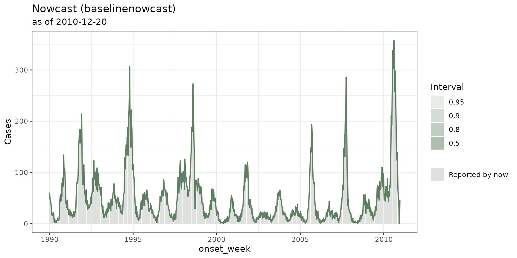
And there is an autoplot() method for a quick look. It is drawn in green, the colour this package reserves for the epidemic process — a nowcast is an estimate of what happened, not of when we found out:

autoplot(baseline)

A green fan chart of the dengue nowcast: nested prediction intervals around a median line, with the counts reported so far as points.

Strata are handled for you

When the tbl_now declares strata, run_nowcast() does whatever that backend needs to honour them — one reporting triangle per stratum for baselinenowcast, NobBS.strat() instead of NobBS(), one fit per stratum for surveillance, regional_epinow() instead of estimate_infections() — and the stratum ends up as an ordinary column of the output:

dengue_by_sex <- denguedat |>
  filter(onset_week >= as.Date("2008-01-01")) |>
  count(onset_week, report_week, gender, name = "n") |>
  tbl_now(
    event_date = onset_week, report_date = report_week, case_count = n,
    strata = gender, data_type = "count-incidence", verbose = FALSE
  ) |>
  filter(report_week <= now) |>
  change_now(now = now)

by_sex <- run_nowcast(dengue_by_sex, "baselinenowcast", draws = 1000, verbose = FALSE)

as_tibble(by_sex)

#> # A tibble: 2,556 × 4
#>    onset_week gender .quantile_level .value
#>    <date>     <chr>            <dbl>  <dbl>
#>  1 2008-01-07 Female           0.025      9
#>  2 2008-01-07 Female           0.05       9
#>  3 2008-01-07 Female           0.1        9
#>  4 2008-01-07 Female           0.25       9
#>  5 2008-01-07 Female           0.5        9
#>  6 2008-01-07 Female           0.75       9
#>  7 2008-01-07 Female           0.9        9
#>  8 2008-01-07 Female           0.95       9
#>  9 2008-01-07 Female           0.975      9
#> 10 2008-01-07 Male             0.025     13
#> # ℹ 2,546 more rows

tidy() labels each block with its stratum, so (stratum, event_date) is a unique key and the two series can never be confused for one another:

tidy(by_sex)

#> # A tibble: 284 × 7
#>    event_date stratum estimate conf.low conf.high level engine         
#>    <date>     <chr>      <dbl>    <dbl>     <dbl> <dbl> <chr>          
#>  1 2008-01-07 Female         9        9         9  0.95 baselinenowcast
#>  2 2008-01-14 Female         9        9         9  0.95 baselinenowcast
#>  3 2008-01-21 Female         3        3         3  0.95 baselinenowcast
#>  4 2008-01-28 Female         4        4         4  0.95 baselinenowcast
#>  5 2008-02-04 Female         3        3         3  0.95 baselinenowcast
#>  6 2008-02-11 Female         2        2         2  0.95 baselinenowcast
#>  7 2008-02-18 Female         3        3         3  0.95 baselinenowcast
#>  8 2008-02-25 Female         5        5         5  0.95 baselinenowcast
#>  9 2008-03-10 Female         1        1         1  0.95 baselinenowcast
#> 10 2008-03-17 Female         1        1         1  0.95 baselinenowcast
#> # ℹ 274 more rows

If a backend genuinely cannot stratify, it warns and pools rather than pretending.

2. Scoring a nowcast

score_nowcast() compares the predictive quantiles with what was eventually observed, using the weighted interval score (WIS) of Bracher et al. (2021), plus the absolute error of the median and the 50% and 90% interval coverage.

Scoring only makes sense against data the model had not seen, which is why snapshot was truncated at now and the truth comes from the full series:

score_nowcast(baseline, truth = dengue)

#> # A tibble: 144 × 7
#>    .method         onset_week .observed   wis ae_median coverage_50 coverage_90
#>    <chr>           <date>         <int> <dbl>     <dbl> <lgl>       <lgl>      
#>  1 baselinenowcast 2008-01-07        22     0         0 TRUE        TRUE       
#>  2 baselinenowcast 2008-01-14        19     0         0 TRUE        TRUE       
#>  3 baselinenowcast 2008-01-21         8     0         0 TRUE        TRUE       
#>  4 baselinenowcast 2008-01-28        14     0         0 TRUE        TRUE       
#>  5 baselinenowcast 2008-02-04         5     0         0 TRUE        TRUE       
#>  6 baselinenowcast 2008-02-11         5     0         0 TRUE        TRUE       
#>  7 baselinenowcast 2008-02-18         4     0         0 TRUE        TRUE       
#>  8 baselinenowcast 2008-02-25        11     0         0 TRUE        TRUE       
#>  9 baselinenowcast 2008-03-03         2     0         0 TRUE        TRUE       
#> 10 baselinenowcast 2008-03-10         2     0         0 TRUE        TRUE       
#> # ℹ 134 more rows

Lower WIS is better; coverage_90 should be TRUE about nine times in ten if the intervals are honest.

If you would rather use the full score suite, as_scoringutils() reshapes the same object into the format it expects:

baseline |>
  as_scoringutils(truth = dengue) |>
  scoringutils::as_forecast_quantile() |>
  scoringutils::score()

tbl.now’s own wis and the one computes agree to machine precision — the package’s test suite checks exactly that, on the same numbers, rather than trusting either implementation on its own.

3. Ensembles

Models fail in different directions, and combining them cancels part of that: an ensemble is rarely the single best model, but it is also rarely the worst, which is worth a great deal when you have to commit to something before you know which epidemic you are facing. How you combine them matters more than most write-ups admit, and the two rules below behave differently enough that the choice is worth making deliberately. Because every run_nowcast() result has the same shape, combining them is one call.

The members below are the fits from the cards above, so nothing is refitted:

members <- list(
  baselinenowcast   = baseline,
  diseasenowcasting = dnc,
  # The SAME package, a different epidemic process. An ensemble is not only a
  # hedge across packages -- two structurally different models from one package
  # disagree in their own way, and that disagreement is worth combining too.
  dnc_ar1           = run_nowcast(
    snapshot,
    engine_diseasenowcasting(
      model = diseasenowcasting::model(
        epidemic = diseasenowcasting::ar1_epidemic()
      ),
      label = "dnc_ar1"
    )
  ),
  epinowcast        = enw,
  NobBS             = nobbs,
  EpiNow2           = en2
)

ensemble <- nowcast_ensemble(members)

#> -- A <tbl_nowcast> from method "ensemble" --------------------------------------
#> * now: "2010-10-04"
#> * event dates: 10
#> * quantile levels: 0.025, 0.05, 0.1, 0.25, 0.5, 0.75, 0.9, 0.95, and 0.975
#> * draws: none (quantiles only)
#> # A tibble: 6 x 3
#>   onset_week .quantile_level .value
#>   <date>               <dbl>  <dbl>
#> 1 2010-08-02           0.025   324.
#> 2 2010-08-02           0.05    324.
#> 3 2010-08-02           0.1     324.
#> 4 2010-08-02           0.25    354.
#> 5 2010-08-02           0.5     354.
#> 6 2010-08-02           0.75    354.
#> i 84 more rows. Use `as_tibble()` for all of them.

The ensemble against its parts

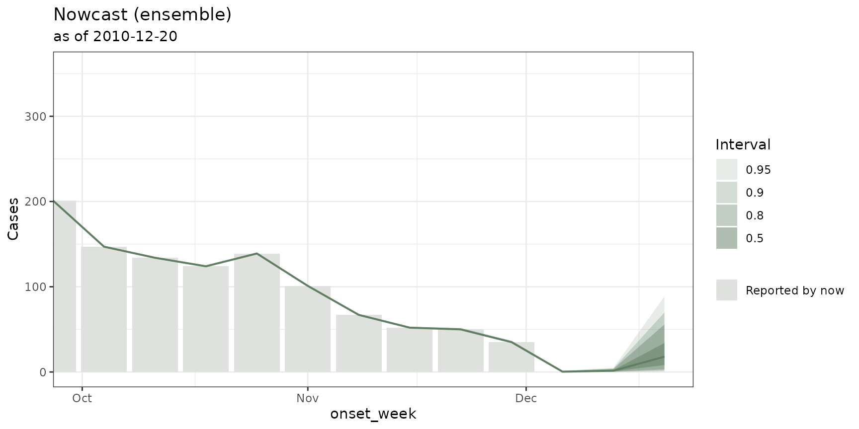
The reason to build one is easier to see than to describe. Each thin line below is one member’s median, the green fan is the ensemble, and the dashed line is what those weeks eventually reached. The window is the ensemble’s own: it keeps only the dates every member covers, and epinowcast reports just the reference dates it is nowcasting.

Coloured lines, one per member, fan out over the final weeks; the ensemble's shaded band sits among them and its median tracks the eventual truth more closely than most single members.

The quantile ensemble against each of its members over the last weeks before now.

Three things are worth reading off it.

Most members fan out at the now edge and lie on top of each other before it. That is the shape of the problem: the settled weeks have nothing left to nowcast, so any sane model reproduces them, and the disagreement concentrates exactly where the answer is not yet known. The spread at the right is what an ensemble exists to absorb.

EpiNow2 is the exception, and it disagrees everywhere. It is not estimating the same thing as the others: it fits a latent infection curve and reports the smooth implied by it, rather than correcting each week’s reported count for its outstanding delay. A member that is off by a constant factor on settled weeks is usually a sign of that kind of mismatch rather than of a bad fit.

And the ensemble’s median sits inside the spread rather than at either edge of it. That is the entire trade: it is rarely the best line on any given week, and it is rarely the worst either — which is worth a great deal when you have to commit before knowing which member was right.

An ensemble reports only what every member can. The fan above has as many bands as the levels its members share, and here that is all nine of nowcast_quantile_levels() — every member either keeps draws or was asked for those levels at fit time. Add surveillance, which keeps none and reports a fixed {0.025, 0.5, 0.975}, and the fan collapses to a single 95% band. That is why it is a card above but not a member here — see the note below.

These fits use approximate inference. epinowcast runs through enw_pathfinder() and EpiNow2 through stan_opts(method = "pathfinder") so this article rebuilds in minutes rather than overnight. That is fine for showing how the ensemble machinery behaves and is not a tuned posterior for either model — do not read any single member’s band as that package’s considered answer.

An ensemble is a tbl_nowcast like any other, so it scores, plots and tidies the same way. Its engine is the ensemble’s name rather than a package:

tidy(ensemble)

#> # A tibble: 10 × 7
#>    event_date stratum estimate conf.low conf.high level engine  
#>    <date>     <chr>      <dbl>    <dbl>     <dbl> <dbl> <chr>   
#>  1 2010-08-02 all         354.     324.      355.  0.95 ensemble
#>  2 2010-08-09 all         354.     354.      364.  0.95 ensemble
#>  3 2010-08-16 all         361.     361.      370.  0.95 ensemble
#>  4 2010-08-23 all         252.     252.      264.  0.95 ensemble
#>  5 2010-08-30 all         282.     282       300.  0.95 ensemble
#>  6 2010-09-06 all         289.     283       292.  0.95 ensemble
#>  7 2010-09-13 all         267.     264.      292.  0.95 ensemble
#>  8 2010-09-20 all         257.     245.      320.  0.95 ensemble
#>  9 2010-09-27 all         229.     179.      402.  0.95 ensemble
#> 10 2010-10-04 all         226.     108.      549.  0.95 ensemble

Two ways of combining

type = "quantile" (the default) averages the members’ quantiles level by level — vincentization. It is the workhorse of the forecast hubs, it always applies because every backend produces quantiles, and it tends to produce narrower intervals than the members.

type = "linear_pool" instead pools the members’ draws into a mixture distribution and re-summarises it. It needs draws from every member and generally produces wider intervals, because disagreement between models becomes extra spread rather than being averaged away.

sharp <- nowcast_ensemble(members, type = "quantile")

# The pool needs draws, so it takes the members that have them.
with_draws <- members[c("baselinenowcast", "diseasenowcasting",
                        "dnc_ar1", "epinowcast")]
wide <- nowcast_ensemble(with_draws, type = "linear_pool", n_draws = 4000)

Which one you want depends on whether you read between-model disagreement as noise to be averaged out (quantile) or as genuine uncertainty to be propagated (linear pool).

The linear pool needs draws, and not every backend has them. Of the six engines above, baselinenowcast, diseasenowcasting, epinowcast and EpiNow2 keep per-event-date draws; NobBS and surveillance report summaries only. (NobBS’s nowcast.post.samps cover the now date rather than every event date, which is not the same thing.) type = "linear_pool" refuses a set of members that includes one of the two, rather than silently dropping it and returning a differently-composed ensemble under the same name — which is why the call above selects its members explicitly.

Members must agree on what they are predicting. An ensemble combines members target by target, so a date one member covers and another does not cannot be combined: averaging over whoever happens to be present would report a single member’s own value as the ensemble’s. Those targets are dropped, with a warning saying how many. This is not hypothetical — EpiNow2 forecasts one period past the end of the data, and before run_nowcast() trimmed it that lone extra week landed exactly at the now edge, which is the part of the picture people read.

Why surveillance is not a member here. There is a principled reason, and it is arithmetic. surveillance keeps no per-date draws and reports a fixed {0.025, 0.5, 0.975}, so it cannot be asked for any other level after the fit. An ensemble reports only the levels every member carries, so adding it drops the ensemble from the nine hub levels to those three — one 95% band instead of a fan — and every other member’s extra resolution is thrown away to accommodate one that has none.

nowcast_ensemble() warns when this happens rather than pretending. The fix is at fit time: leave it out, or widen what it reports where the package lets you (surveillance’s control$alpha). Nothing in nowcast_ensemble() treats it specially.

Weights

By default every member counts the same. You can also give weights directly:

nowcast_ensemble(members, weights = c(
  baselinenowcast = 0.3, diseasenowcasting = 0.2, dnc_ar1 = 0.1,
  epinowcast = 0.2, NobBS = 0.1, EpiNow2 = 0.1
))

or learn them from how the members actually performed. nowcast_backtest() walks back through time: at each retrospective date it truncates the data to the reports available then, refits every method, and scores the result against what was eventually observed.

It takes the same engines you fitted with, so there is no second place to keep the arguments in step. An engine’s label becomes its name in the result — which is how one package appears twice, so the two diseasenowcasting models above can be weighted separately rather than sharing one weight:

backtest <- nowcast_backtest(
  dengue,
  engine_baselinenowcast(draws = 1000),
  engine_diseasenowcasting(),
  engine_diseasenowcasting(
    model = diseasenowcasting::model(
      epidemic = diseasenowcasting::ar1_epidemic()
    ),
    label = "dnc_ar1"
  ),
  engine_nobbs(max_D = 10, moving_window = 64),
  now_dates = now - 7 * 8 * (3:1),
  seed      = 20260824
)

tidy(backtest)

#> # A tibble: 6 × 9
#>   method now        event_date stratum observed   wis ae_median coverage_50
#>   <chr>  <date>     <date>     <chr>      <dbl> <dbl>     <dbl> <lgl>      
#> 1 NobBS  2010-04-19 2009-02-02 all           48     0         0 TRUE       
#> 2 NobBS  2010-04-19 2009-02-09 all           47     0         0 TRUE       
#> 3 NobBS  2010-04-19 2009-02-16 all           43     0         0 TRUE       
#> 4 NobBS  2010-04-19 2009-02-23 all           42     0         0 TRUE       
#> 5 NobBS  2010-04-19 2009-03-02 all           24     0         0 TRUE       
#> 6 NobBS  2010-04-19 2009-03-09 all           27     0         0 TRUE       
#> # ℹ 1 more variable: coverage_90 <lgl>

Why not every ensemble member is backtested here. A backtest is length(methods) × length(now_dates) model fits. epinowcast and EpiNow2 are both Stan models and each would add three more, so they are left out of this backtest to keep the article buildable — not because anything stops them. If you weight an ensemble from a backtest that does not cover every member, give the uncovered ones weights yourself; nowcast_ensemble() will not invent them.

tidy() on a backtest gives one row per (method, now date, target), which goes straight into dplyr or ggplot2:

#> # A tibble: 3 × 4
#>   method            mean_wis mean_ae_median coverage_90
#>   <chr>                <dbl>          <dbl>       <dbl>
#> 1 diseasenowcasting     0.5            0.97        0.99
#> 2 baselinenowcast       0.7            1.39        0.99
#> 3 NobBS                 1.91           2.86        0.97

This is the expensive part of the workflow — it is length(methods) × length(now_dates) model fits — so keep now_dates short when the members are Bayesian. Pass seed so the backtest is reproducible: one set.seed() before the whole thing only pins anything if every method draws the same random numbers in the same order, which stops being true the moment you drop a method.

From the backtest, nowcast_weights() offers two rules:

fitted_weights <- nowcast_weights(backtest, type = "inverse_score")
fitted_weights                                    # w proportional to 1 / mean WIS

nowcast_weights(backtest, type = "optim")         # w minimising the ensemble's WIS

#>             NobBS   baselinenowcast diseasenowcasting 
#>             0.132             0.360             0.508

"inverse_score" is the safe default: it is monotone in performance, never collapses onto a single model, and cannot overfit. "optim" searches the simplex for the weights that would have minimised the ensemble’s WIS over the training window; it is better in principle, but with only a handful of retrospective dates it happily overfits, so prefer it when the training window is long.

Either rule plugs straight into the ensemble:

nowcast_ensemble(members, weights = "inverse_score", backtest = backtest)

4. Adding your own model

This is the part that makes the whole thing worth building. A back-end is two S3 methods, and they can live in your own package, your analysis script, or a one-off chunk. Nothing inside tbl.now needs to change.

run_nowcast(x, method = "mymodel") builds a little object of class c("mymodel", "nowcast_method") and calls

nowcast_fit(method, x, ...) — run the model, return whatever it returns;
nowcast_tidy(method, fit, x, ..., quantile_levels) — describe the result as predictions (one row per event date, stratum and quantile level) or draws (one row per event date, stratum and draw). Either may be NULL, not both.

vignette("custom-nowcast-models") is the full account: what your method may assume about the tbl_now it is handed, how to reuse the converters instead of reshaping by hand, a complete worked back-end that needs no modelling package, and what shipping one in a package involves.

Learning more

Introduction vignette: https://rodrigozepeda.github.io/tbl.now/articles/tbl.now.html for the full anatomy of a tbl_now, data types, and temporal effects.
End-to-end tutorial on real, messy surveillance data — cleaning, diagnostics and nowcasting: https://rodrigozepeda.github.io/tbl.now/articles/example.html
Tutorial on diagnosing your dataset — what is in it, what is structurally wrong with it, and detecting batches and other reporting-delay artifacts: https://rodrigozepeda.github.io/tbl.now/articles/diagnosing-a-tbl-now.html
Using different nowcasting engines for the same dataset: https://rodrigozepeda.github.io/tbl.now/articles/nowcasting-models.html
Ensemble nowcasting across different engines https://rodrigozepeda.github.io/tbl.now/articles/ensemble-nowcasting.html
Adding your own nowcasting model https://rodrigozepeda.github.io/tbl.now/articles/custom-nowcast-models.html
Package reference: https://rodrigozepeda.github.io/tbl.now/reference/

References

Bracher, Johannes, Evan L. Ray, Tilmann Gneiting, and Nicholas G. Reich. 2021. “Evaluating Epidemic Forecasts in an Interval Format.” PLoS Computational Biology 17 (2): e1008618. https://doi.org/10.1371/journal.pcbi.1008618.