tbl.now

Within R, the tidyverse ecosystem (Wickham et al. 2019) provides a widely adopted framework for data analysis. In this paradigm, data is structured such that rows represent individual observations and columns represent variables. This approach is commonly referred to as tidy data (Wickham 2014).

Several tidyverse extensions exist for working with time series data, including tsibble, tibbletime, and timetk (Wang et al. 2020; Wang 2019; Dancho and Vaughan 2023). These packages provide time-aware tibbles and tools that integrate smoothly with the tidyverse. However, epidemiological nowcasting requires two time indices simultaneously: an event time and a reporting time. Classical time-series abstractions assume only a single index and therefore do not fully support this structure.

The tbl.now class and package addresses this gap. The tbl.now extends a regular tibble() to explicitly encode epidemiological event and report dates, allowing consistent data transformation, delay computation, and integration with the diseasenowcasting modeling workflow.

More concretely, tbl.now was designed to:

Standardize the data inputs required by diseasenowcasting models.
Preserve tidyverse compatibility so users can continue to apply familiar dplyr operations.
Diagnose reporting artefacts directly from the data — reporting-delay drift and change points (test_delay_drift(), test_delay_changepoint()) and batch (backlog) reporting (detect_report_batches()).
Facilitate seamless integration into iterative modeling workflows (Gelman et al. 2020; Wickham et al. 2023):

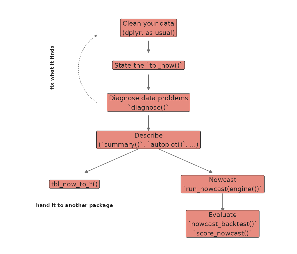
Data Cleaning -> Modeling -> New Data Cleaning -> New Modeling -> ...

We’ll begin by loading the required packages:

library(dplyr, quietly = TRUE)
library(lubridate)
library(tbl.now)

The `tbl.now` Framework

In an epidemiological nowcast, we typically observe two key dates:

event_date: when the underlying event occurred (e.g., symptom onset, exposure, sample collection).
report_date: when the event was recorded in the data system (e.g., lab result processed, clinical visit documented).

The nowcasting task is:

To estimate, for each past event_date, how many events have already occurred but have not yet been reported as of now. That is, the nowcast will predict how many observations will eventually be observed for the event_dates.

A tbl.now object is therefore a specialized tibble() that:

Identifies the event_date and report_date columns.
Stores these as attributes to enable consistent processing.
Automatically computes auxiliary fields such as delay, numerical indices, and frequency units.
Ensures the dataset is well-formed for downstream diseasenowcasting models.

Example

Consider the following dataset:

df <- data.frame(
  symptom_onset = c(ymd("2023/12/25"), ymd("2023/12/26"), ymd("2023/12/25"), ymd("2023/12/26")),
  medical_visit = c(ymd("2023/12/26"), ymd("2023/12/26"), ymd("2023/12/27"), ymd("2023/12/27")),
  n = c(10, 2, 5, 11)
)

knitr::kable(df, caption = "Example dataset")

Example dataset
symptom_onset	medical_visit	n
2023-12-25	2023-12-26	10
2023-12-26	2023-12-26	2
2023-12-25	2023-12-27	5
2023-12-26	2023-12-27	11

Here:

symptom_onset is the event date.
medical_visit is the report date.
n is the number of reported cases for each event–report combination.

We can convert this into a tbl_now():

df |>
  tbl_now(event_date = symptom_onset, report_date = medical_visit, case_count = n)
#> ℹ Identified data as <count-incidence> with counts in column "n".
#> # A tibble:  4 × 6
#> # Data type: "count-incidence"
#> # Frequency: Event: `days` | Report: `days`
#>   symptom_onset medical_visit       n .event_num .report_num .delay
#>   <date>        <date>          <dbl>      <dbl>       <dbl>  <dbl>
#>   [event_date]  [report_date] [cases]      [...]       [...]  [...]
#> 1 2023-12-25    2023-12-26         10          0           1      1
#> 2 2023-12-26    2023-12-26          2          1           1      0
#> 3 2023-12-25    2023-12-27          5          0           2      2
#> 4 2023-12-26    2023-12-27         11          1           2      1
#> # ────────────────────────────────────────────────────────────────────────────────
#> # Now: 2023-12-27 | Event date: "symptom_onset" | Report date: "medical_visit"
#> # ────────────────────────────────────────────────────────────────────────────────

This performs several operations automatically:

Detects the data type (count-incidence in this example).
Infers the frequency units of event and report dates (daily).
Tags the correct columns as event_date, report_date, and case_count.
Computes .event_num, .report_num, and .delay columns.
Identifies the appropriate now date (the most recent report date).

The remaining sections describe these features and the broader tbl.now toolkit.

Attributes of a tbl_now()

A tbl_now() stores information about its structure using object attributes, ensuring consistent behavior across transformations and modeling steps. The primary attributes are:

now: the “current” reporting date used for nowcasting, typically the most recent report_date.
event_date: the column name storing event dates.
report_date: the column name storing report dates.
event_units: the temporal units for event dates (e.g., “days”, “weeks”, “numeric”).
report_units: the temporal units for report dates.
data_type: one of the following (see the data types section):
- linelist
- count-incidence
- count-cumulative.
strata (optional)¹: variables for which the nowcast should be computed separately (e.g., age group, sex).
covariates (optional): predictor variables that may improve the nowcast (e.g., weather covariates).
is_censored (optional): identifies cases where some reports arrive in artificial “batches” representing right-censoring rather than true reporting dynamics (e.g. when there is a system error and reports from a lab are not registered until a week after)
case_count (optional): the column storing case counts when the dataset is aggregated.
temporal_effects (optional): a lazy specification (list of temporal_effects() configs) stored via add_temporal_effects(). Columns are only materialised when compute_temporal_effects() is called. See the temporal effects section for more details.

You can access any attribute using the corresponding getter, e.g. get_event_date() or get_strata().

Data types

A tbl_now() can represent one of three data structures:

Linelist: Each row corresponds to a single reported observation.

Linelist data
patient	event_date	report_date	.event_num	.report_num	.delay
1	2020-09-12	2020-09-12	0	0	0
2	2020-09-12	2020-09-12	0	0	0
3	2020-09-12	2020-09-13	0	1	1
4	2020-09-13	2020-09-13	1	1	0
5	2020-09-13	2020-09-13	1	1	0
6	2020-09-13	2020-09-13	1	1	0

Count-incidence: Each row summarizes how many events with a given event_date were reported exactly on that report_date.

Count-incidence data
n	event_date	report_date	.event_num	.report_num	.delay
7	2020-09-12	2020-09-12	0	0	0
1	2020-09-12	2020-09-13	0	1	1
9	2020-09-12	2020-09-14	0	2	2
5	2020-09-13	2020-09-13	1	1	0
0	2020-09-13	2020-09-14	1	2	1
2	2020-09-13	2020-09-15	1	3	2

Count-cumulative Each row summarizes how many events with a given event_date had been reported up to and including that report_date. The distinction is crucial for nowcasting models that operate either on daily increments or cumulative totals.

Count-cumulative data
n	event_date	report_date	.event_num	.report_num	.delay
1	2020-09-12	2020-09-12	0	0	0
5	2020-09-12	2020-09-13	0	1	1
8	2020-09-12	2020-09-14	0	2	2
2	2020-09-13	2020-09-13	1	1	0
2	2020-09-13	2020-09-14	1	2	1
4	2020-09-13	2020-09-15	1	3	2

The to_count() function allows you to easily convert between different data-types.

Converting Between Data Types

The to_count() function supports structured transformations:

Linelist → Count-Incidence: Aggregates by event–report date, counting only cases reported on that date.

df_linelist |>
  to_count(to = "count-incidence")
#> # A tibble:  3 × 6
#> # Data type: "count-incidence"
#> # Frequency: Event: `days` | Report: `days`
#>   event_date   report_date   .event_num .report_num       n .delay
#>   <date>       <date>             <dbl>       <dbl>   <int>  <dbl>
#>   [event_date] [report_date]      [...]       [...] [cases]  [...]
#> 1 2020-09-12   2020-09-12             0           0       2      0
#> 2 2020-09-12   2020-09-13             0           1       1      1
#> 3 2020-09-13   2020-09-13             1           1       3      0
#> # ────────────────────────────────────────────────────────────────────────────────
#> # Now: 2020-09-13 | Event date: "event_date" | Report date: "report_date"
#> # ────────────────────────────────────────────────────────────────────────────────

Linelist → Count-Cumulative: Aggregates by event–report date, producing cumulative counts up to each report date.

df_linelist |>
  to_count(to = "count-cumulative")
#> # A tibble:  3 × 6
#> # Data type: "count-cumulative"
#> # Frequency: Event: `days` | Report: `days`
#>   event_date   report_date   .event_num .report_num       n .delay
#>   <date>       <date>             <dbl>       <dbl>   <int>  <dbl>
#>   [event_date] [report_date]      [...]       [...] [cases]  [...]
#> 1 2020-09-12   2020-09-12             0           0       2      0
#> 2 2020-09-12   2020-09-13             0           1       3      1
#> 3 2020-09-13   2020-09-13             1           1       3      0
#> # ────────────────────────────────────────────────────────────────────────────────
#> # Now: 2020-09-13 | Event date: "event_date" | Report date: "report_date"
#> # ────────────────────────────────────────────────────────────────────────────────

Note In the previous example the n counts 3 as it is aggregating the 1 observed at report_date = 2020-09-13 and the 2 observed at report_date = 2020-09-12. This is the difference between the count-incidence that specifies the ones observed exactly on that date and the count-cumulative that specifies the ones observed up until and including that date.

Count-Incidence → Count-Cumulative: Computes cumulative sums for each event date across report dates.

df_count_inc |>
  to_count(to = "count-cumulative")
#> # A tibble:  6 × 6
#> # Data type: "count-cumulative"
#> # Frequency: Event: `days` | Report: `days`
#>   event_date   report_date   .event_num .report_num       n .delay
#>   <date>       <date>             <dbl>       <dbl>   <dbl>  <dbl>
#>   [event_date] [report_date]      [...]       [...] [cases]  [...]
#> 1 2020-09-12   2020-09-12             0           0       7      0
#> 2 2020-09-12   2020-09-13             0           1       8      1
#> 3 2020-09-12   2020-09-14             0           2      17      2
#> 4 2020-09-13   2020-09-13             1           1       5      0
#> 5 2020-09-13   2020-09-14             1           2       5      1
#> 6 2020-09-13   2020-09-15             1           3       7      2
#> # ────────────────────────────────────────────────────────────────────────────────
#> # Now: 2020-09-15 | Event date: "event_date" | Report date: "report_date"
#> # ────────────────────────────────────────────────────────────────────────────────

Aggregation within the same type: The to_count() may also be used to re-aggregate datasets that contain duplicate event–report pairs. This is useful when raw surveillance feeds contain repeated entries such as in this case:

df_example <- data.frame(
  n = c(8, 11, 0, 1, 1, 5, 2, 4, 1, 10, 9, 11, 3, 1),
  sex = c(rep("M", 3), rep("F", 4), rep("M", 2), rep("F", 5)),
  event_date = c(
    rep(ymd("2020/09/12"), 3),
    rep(ymd("2020/09/12"), 4),
    rep(ymd("2020/09/13"), 2),
    rep(ymd("2020/09/13"), 5)
  ),
  report_date = c(
    ymd("2020/09/12"), ymd("2020/09/13"), ymd("2020/09/14"),
    ymd("2020/09/12"), ymd("2020/09/13"), ymd("2020/09/14"),
    ymd("2020/09/15"), ymd("2020/09/13"), ymd("2020/09/14"),
    ymd("2020/09/13"), ymd("2020/09/14"),
    ymd("2020/09/15"), ymd("2020/09/16"), ymd("2020/09/17")
  )
)

tbl_example <- df_example |>
  tbl_now(
    event_date = event_date, report_date = report_date,
    data_type = "count-incidence", case_count = n, verbose = FALSE,
    warn_non_uniqueness = FALSE
  )

tbl_example
#> # A tibble:  14 × 7
#> # Data type: "count-incidence"
#> # Frequency: Event: `days` | Report: `days`
#>          n sex   event_date   report_date   .event_num .report_num .delay
#>      <dbl> <chr> <date>       <date>             <dbl>       <dbl>  <dbl>
#>    [cases] [...] [event_date] [report_date]      [...]       [...]  [...]
#>  1       8 M     2020-09-12   2020-09-12             0           0      0
#>  2      11 M     2020-09-12   2020-09-13             0           1      1
#>  3       0 M     2020-09-12   2020-09-14             0           2      2
#>  4       1 F     2020-09-12   2020-09-12             0           0      0
#>  5       1 F     2020-09-12   2020-09-13             0           1      1
#>  6       5 F     2020-09-12   2020-09-14             0           2      2
#>  7       2 F     2020-09-12   2020-09-15             0           3      3
#>  8       4 M     2020-09-13   2020-09-13             1           1      0
#>  9       1 M     2020-09-13   2020-09-14             1           2      1
#> 10      10 F     2020-09-13   2020-09-13             1           1      0
#> 11       9 F     2020-09-13   2020-09-14             1           2      1
#> 12      11 F     2020-09-13   2020-09-15             1           3      2
#> 13       3 F     2020-09-13   2020-09-16             1           4      3
#> 14       1 F     2020-09-13   2020-09-17             1           5      4
#> # ────────────────────────────────────────────────────────────────────────────────
#> # Now: 2020-09-17 | Event date: "event_date" | Report date: "report_date"
#> # ────────────────────────────────────────────────────────────────────────────────

This dataset intentionally contains repeated event_date–report_date pairs within each stratum. If the user wants to aggregate redundant rows, the to_count() function can be used to collapse duplicates by summing the case_count column.

tbl_example |>
  to_count(to = "count-incidence")
#> # A tibble:  9 × 6
#> # Data type: "count-incidence"
#> # Frequency: Event: `days` | Report: `days`
#>   event_date   report_date   .event_num .report_num       n .delay
#>   <date>       <date>             <dbl>       <dbl>   <dbl>  <dbl>
#>   [event_date] [report_date]      [...]       [...] [cases]  [...]
#> 1 2020-09-12   2020-09-12             0           0       9      0
#> 2 2020-09-12   2020-09-13             0           1      12      1
#> 3 2020-09-12   2020-09-14             0           2       5      2
#> 4 2020-09-12   2020-09-15             0           3       2      3
#> 5 2020-09-13   2020-09-13             1           1      14      0
#> 6 2020-09-13   2020-09-14             1           2      10      1
#> 7 2020-09-13   2020-09-15             1           3      11      2
#> 8 2020-09-13   2020-09-16             1           4       3      3
#> 9 2020-09-13   2020-09-17             1           5       1      4
#> # ────────────────────────────────────────────────────────────────────────────────
#> # Now: 2020-09-17 | Event date: "event_date" | Report date: "report_date"
#> # ────────────────────────────────────────────────────────────────────────────────

The function ensures that:

Rows are grouped by event_date, report_date, and any strata, and is_censored.
The case_count column is summed within each group.
Attributes are preserved so the resulting object remains a valid tbl_now.

Temporal effects

Often, temporal covariates improve nowcasting performance by helping adjust for systematic changes occurring within the calendar cycle (e.g., day-of-week effects, seasonal effects, or reporting artefacts). The temporal_effects() function creates a specification (recipe) of the features to compute:

library(almanac)

t_eff <- temporal_effects(
  day_of_week  = TRUE,
  week_of_year = TRUE,
  holidays     = cal_us_federal()
)
t_eff
#> 
#> ── Temporal Effects ────────────────────────────────────────────────────────────
#> The following effects are in place:
#> • "day_of_week"
#> • "week_of_year"
#> • "holidays":
#>   1. New Year's Day, US Martin Luther King Jr. Day, US Presidents' Day, US
#>   Memorial Day, US Juneteenth, US Independence Day, US Labor Day, US Indigenous
#>   Peoples' Day, US Veterans Day, US Thanksgiving, and Christmas

Note that the holidays calendar is an rcalendar object from the almanac package.

Lazy evaluation: attach first, compute later

Temporal effects in tbl.now follow a lazy evaluation pattern:

Attach the spec with add_temporal_effects() (or via the t_effects argument of tbl_now()). This records what should be computed but adds no columns yet.
Materialise the columns with compute_temporal_effects() when you are ready to use them in a model.

data("denguedat")

# Step 1 — create the tbl_now and attach the spec (no columns added yet)
df_now <- denguedat |>
  tbl_now(
    event_date = onset_week, report_date = report_week,
    verbose = FALSE, strata = gender
  )

df_now <- df_now |>
  add_temporal_effects(t_eff)

# The footer shows "T. effects (lazy): ..." — spec is recorded but not computed
df_now
#> # A tibble:  52,987 × 6
#> # Data type: "linelist"
#> # Frequency: Event: `weeks` | Report: `weeks`
#>    onset_week   report_week   gender   .event_num .report_num .delay
#>    <date>       <date>        <chr>         <dbl>       <dbl>  <dbl>
#>    [event_date] [report_date] [strata]      [...]       [...]  [...]
#>  1 1990-01-01   1990-01-01    Male              0           0      0
#>  2 1990-01-01   1990-01-01    Female            0           0      0
#>  3 1990-01-01   1990-01-01    Female            0           0      0
#>  4 1990-01-01   1990-01-08    Female            0           1      1
#>  5 1990-01-01   1990-01-08    Male              0           1      1
#>  6 1990-01-01   1990-01-15    Female            0           2      2
#>  7 1990-01-01   1990-01-15    Female            0           2      2
#>  8 1990-01-01   1990-01-15    Female            0           2      2
#>  9 1990-01-01   1990-01-22    Female            0           3      3
#> 10 1990-01-01   1990-01-08    Female            0           1      1
#> # ────────────────────────────────────────────────────────────────────────────────
#> # Now: 2010-12-20 | Event date: "onset_week" | Report date: "report_week"
#> # Strata: "gender"
#> # T. effects (lazy): [event_date] day_of_week, week_of_year, holidays
#> # ────────────────────────────────────────────────────────────────────────────────
#> # ℹ 52,977 more rows

The footer now shows the spec with (lazy) to signal that the columns have not been computed yet. No new columns appear in the tibble at this point.

# Step 2 — materialise the columns when needed
df_computed <- compute_temporal_effects(df_now)

# Columns are now present and annotated [t_effect]
df_computed
#> # A tibble:  52,987 × 9
#> # Data type: "linelist"
#> # Frequency: Event: `weeks` | Report: `weeks`
#>    onset_week   report_week   gender   .event_num .report_num .delay
#>    <date>       <date>        <chr>         <dbl>       <dbl>  <dbl>
#>    [event_date] [report_date] [strata]      [...]       [...]  [...]
#>  1 1990-01-01   1990-01-01    Male              0           0      0
#>  2 1990-01-01   1990-01-01    Female            0           0      0
#>  3 1990-01-01   1990-01-01    Female            0           0      0
#>  4 1990-01-01   1990-01-08    Female            0           1      1
#>  5 1990-01-01   1990-01-08    Male              0           1      1
#>  6 1990-01-01   1990-01-15    Female            0           2      2
#>  7 1990-01-01   1990-01-15    Female            0           2      2
#>  8 1990-01-01   1990-01-15    Female            0           2      2
#>  9 1990-01-01   1990-01-22    Female            0           3      3
#> 10 1990-01-01   1990-01-08    Female            0           1      1
#>    .event_day_of_week .event_week_of_year .event_holiday
#>                 <int>               <int>          <int>
#>            [t_effect]          [t_effect]     [t_effect]
#>  1                  2                   1              1
#>  2                  2                   1              1
#>  3                  2                   1              1
#>  4                  2                   1              1
#>  5                  2                   1              1
#>  6                  2                   1              1
#>  7                  2                   1              1
#>  8                  2                   1              1
#>  9                  2                   1              1
#> 10                  2                   1              1
#> # ────────────────────────────────────────────────────────────────────────────────
#> # Now: 2010-12-20 | Event date: "onset_week" | Report date: "report_week"
#> # Strata: "gender"
#> # T. effects: [event_date] day_of_week, week_of_year, holidays
#> # T. effect cols: ".event_day_of_week", ".event_week_of_year", and
#> # ".event_holiday"
#> # ────────────────────────────────────────────────────────────────────────────────
#> # ℹ 52,977 more rows

After compute_temporal_effects():

The effect columns (.event_day_of_week, .event_week_of_year, .event_holiday) are added.
get_temporal_effect_cols() lists them.
The original spec remains accessible via get_temporal_effects(), so you always know which effects were requested even after further dplyr operations.

get_temporal_effects(df_computed) # The spec (list of configs)
#> [[1]]
#> [[1]]$t_effects
#> 
#> ── Temporal Effects ────────────────────────────────────────────────────────────
#> The following effects are in place:
#> • "day_of_week"
#> • "week_of_year"
#> • "holidays":
#>   1. New Year's Day, US Martin Luther King Jr. Day, US Presidents' Day, US
#>   Memorial Day, US Juneteenth, US Independence Day, US Labor Day, US Indigenous
#>   Peoples' Day, US Veterans Day, US Thanksgiving, and Christmas
#> 
#> [[1]]$date_type
#> [1] "event_date"
#> 
#> [[1]]$weekend_days
#> [1] "Sat" "Sun"
get_temporal_effect_cols(df_computed) # The computed column names
#> [1] ".event_day_of_week"  ".event_week_of_year" ".event_holiday"

After-holiday and after-weekend effects

Reporting often rebounds on the first working day(s) after a holiday or a weekend. To capture that, temporal_effects() has holiday_lags and weekend_lags: each takes a depth N and creates indicator columns ..._holiday_lag_1 … ..._holiday_lag_N (and ..._weekend_lag_k) that flag dates falling exactly k working days after a holiday / weekend. Working days skip weekends and other holidays, so the effect lands on the first day back at work.

# Flag the two working days after a holiday, and the working day after a weekend
after_eff <- temporal_effects(
  holidays     = cal_us_federal(),
  holiday_lags = 2,
  weekend_lags = 1
)
after_eff
#> 
#> ── Temporal Effects ────────────────────────────────────────────────────────────
#> The following effects are in place:
#> • "after-holiday" effect: first 2 working days
#> • "after-weekend" effect: first working day
#> • "holidays":
#>   1. New Year's Day, US Martin Luther King Jr. Day, US Presidents' Day, US
#>   Memorial Day, US Juneteenth, US Independence Day, US Labor Day, US Indigenous
#>   Peoples' Day, US Veterans Day, US Thanksgiving, and Christmas

Event- vs report-date effects

By default effects are derived from the event date and named .event_*. Pass date_type = "report_date" to add_temporal_effects() to derive them from the report date instead (columns named .report_*). Both can coexist on the same tbl_now, and every converter carries both sets of columns.

df_now |>
  add_temporal_effects(temporal_effects(week_of_year = TRUE), date_type = "event_date") |>
  add_temporal_effects(temporal_effects(day_of_week = TRUE),  date_type = "report_date")

Modifying a tbl_now() with `dplyr`

A tbl_now()’s attributes can be modified using the functions in add_*, change_*, or remove_*. These functions share a consistent interface that allows users to incrementally manipulate strata, covariates, and temporal effects.

The example below demonstrates how to create a tbl_now(), add strata and temporal effects, later modify the strata, and finally remove the temporal effects.

data("mpoxdat")

df_now <- mpoxdat |>
  tbl_now(
    event_date = dx_date, report_date = dx_report_date,
    case_count = n, verbose = FALSE, strata = race
  )

df_now
#> # A tibble:  1,417 × 7
#> # Data type: "count-incidence"
#> # Frequency: Event: `days` | Report: `days`
#>    dx_date      dx_report_date race              n .event_num .report_num .delay
#>    <date>       <date>         <chr>         <int>      <dbl>       <dbl>  <dbl>
#>    [event_date] [report_date]  [strata]      [cas…      [...]       [...]  [...]
#>  1 2022-07-08   2022-07-12     Asian             4          0           4      4
#>  2 2022-07-08   2022-07-12     Black             6          0           4      4
#>  3 2022-07-08   2022-07-12     Hispanic          6          0           4      4
#>  4 2022-07-08   2022-07-12     Non-Hispanic…     6          0           4      4
#>  5 2022-07-08   2022-07-13     Asian             2          0           5      5
#>  6 2022-07-08   2022-07-13     Black             3          0           5      5
#>  7 2022-07-08   2022-07-13     Hispanic          8          0           5      5
#>  8 2022-07-08   2022-07-13     Non-Hispanic…     5          0           5      5
#>  9 2022-07-08   2022-07-14     Black             1          0           6      6
#> 10 2022-07-08   2022-07-14     Hispanic          3          0           6      6
#> # ────────────────────────────────────────────────────────────────────────────────
#> # Now: 2023-05-19 | Event date: "dx_date" | Report date: "dx_report_date"
#> # Strata: "race"
#> # ────────────────────────────────────────────────────────────────────────────────
#> # ℹ 1,407 more rows

You can see that the strata is race with the corresponding get_*:

get_strata(df_now)
#> [1] "race"

Strata can be modified with the change_* family of functions. The following example adds a new column containing an uppercase version of the existing race variable and sets it as the new strata:

df_now <- df_now |>
  mutate(RACE_UPPER = toupper(race)) |>
  change_strata(RACE_UPPER)

get_strata(df_now)
#> [1] "RACE_UPPER"

To attach a lazy temporal-effects spec, use add_temporal_effects(), then materialise with compute_temporal_effects():

df_now <- df_now |>
  add_temporal_effects(temporal_effects(week_of_year = TRUE))

# Spec is stored (lazy):
get_temporal_effects(df_now)
#> [[1]]
#> [[1]]$t_effects
#> 
#> ── Temporal Effects ────────────────────────────────────────────────────────────
#> The following effects are in place:
#> • "week_of_year"
#> 
#> [[1]]$date_type
#> [1] "event_date"
#> 
#> [[1]]$weekend_days
#> [1] "Sat" "Sun"

# Compute to add columns:
df_now <- compute_temporal_effects(df_now)
get_temporal_effect_cols(df_now)
#> [1] ".event_week_of_year"

Attributes can be removed using the corresponding remove_* functions. remove_temporal_effects() drops both the spec and any computed columns:

df_now <- df_now |>
  remove_temporal_effects() |>
  remove_all_strata()
#> Warning: *Non-unique*: Data has multiple rows for the same event (dx_date) and
#> report(dx_report_date) dates. Consider using `to_count()` to aggregate the data
#> or`distinct()` to remove repeated observations.

df_now
#> # A tibble:  1,417 × 8
#> # Data type: "count-incidence"
#> # Frequency: Event: `days` | Report: `days`
#>    dx_date      dx_report_date race                     n .event_num .report_num
#>    <date>       <date>         <chr>                <int>      <dbl>       <dbl>
#>    [event_date] [report_date]  [...]              [cases]      [...]       [...]
#>  1 2022-07-08   2022-07-12     Asian                    4          0           4
#>  2 2022-07-08   2022-07-12     Black                    6          0           4
#>  3 2022-07-08   2022-07-12     Hispanic                 6          0           4
#>  4 2022-07-08   2022-07-12     Non-Hispanic White       6          0           4
#>  5 2022-07-08   2022-07-13     Asian                    2          0           5
#>  6 2022-07-08   2022-07-13     Black                    3          0           5
#>  7 2022-07-08   2022-07-13     Hispanic                 8          0           5
#>  8 2022-07-08   2022-07-13     Non-Hispanic White       5          0           5
#>  9 2022-07-08   2022-07-14     Black                    1          0           6
#> 10 2022-07-08   2022-07-14     Hispanic                 3          0           6
#>    .delay RACE_UPPER        
#>     <dbl> <chr>             
#>     [...] [...]             
#>  1      4 ASIAN             
#>  2      4 BLACK             
#>  3      4 HISPANIC          
#>  4      4 NON-HISPANIC WHITE
#>  5      5 ASIAN             
#>  6      5 BLACK             
#>  7      5 HISPANIC          
#>  8      5 NON-HISPANIC WHITE
#>  9      6 BLACK             
#> 10      6 HISPANIC          
#> # ────────────────────────────────────────────────────────────────────────────────
#> # Now: 2023-05-19 | Event date: "dx_date" | Report date: "dx_report_date"
#> # ────────────────────────────────────────────────────────────────────────────────
#> # ℹ 1,407 more rows

get_temporal_effects(df_now) # Empty list — no spec
#> list()
get_temporal_effect_cols(df_now) # character(0) — no computed cols
#> character(0)
get_strata(df_now)
#> NULL

Modifying a tbl_now() with dplyr

tbl_now() objects extend tibble(), and therefore support standard dplyr verbs. The class attempts to preserve and adapt its internal attributes when operations are performed. For example, renaming a strata column will automatically update the stored strata attribute.

library(dplyr, quietly = TRUE)
data(denguedat)

df_now <- tbl_now(denguedat,
  event_date = onset_week,
  report_date = report_week, strata = gender,
  verbose = FALSE
)

# Current strata
get_strata(df_now)
#> [1] "gender"

After renaming the column, the strata attribute updates accordingly:

df_now <- df_now |>
  rename(male_or_female = gender)

get_strata(df_now)
#> [1] "male_or_female"

Certain operations may cause a tbl_now() object to drop back to a standard tibble. This occurs when the operation removes necessary structure—for example, collapsing all data into a single row with summarise():

df_now |>
  summarise(number_males = sum(male_or_female == "Male"))
#> Warning: Dropping `tbl_now` attributes and converting to `tibble`
#> # A tibble: 1 × 1
#>   number_males
#>          <int>
#> 1        26395

Updating a tbl_now()

A tbl_now() object can be updated using the update() method with another data.frame, tibble, or tbl_now() as input. When the column structure is compatible, the update process retains the strata, covariate, and temporal-effect attributes from the original object, and recalculates “now” estimates using the combined data.

Below is an example using an initial dataset:

df <- data.frame(
  patient = 1:6,
  event_date = c(rep(ymd("2020/09/12"), 3), rep(ymd("2020/09/13"), 3)),
  report_date = c(
    ymd("2020/09/12"), ymd("2020/09/13"), ymd("2020/09/14"),
    ymd("2020/09/13"), ymd("2020/09/14"), ymd("2020/09/15")
  )
)

df_now <- tbl_now(df,
  event_date = event_date,
  report_date = report_date, verbose = FALSE
)

And a follow-up dataset containing newly reported cases:

df_new <- data.frame(
  patient = 7:13,
  event_date = c(
    ymd("2020/09/13"),
    rep(ymd("2020/09/14"), 3),
    rep(ymd("2020/09/15"), 3)
  ),
  report_date = c(
    ymd("2020/09/14"), ymd("2020/09/14"), ymd("2020/09/15"),
    ymd("2020/09/16"), ymd("2020/09/15"), ymd("2020/09/16"),
    ymd("2020/09/17")
  )
)

We can update the original object by incorporating the new data:

df_updated <- update(df_now, new_data = df_new)

df_updated
#> # A tibble:  13 × 6
#> # Data type: "linelist"
#> # Frequency: Event: `days` | Report: `days`
#>    patient event_date   report_date   .event_num .report_num .delay
#>      <int> <date>       <date>             <dbl>       <dbl>  <dbl>
#>      [...] [event_date] [report_date]      [...]       [...]  [...]
#>  1       1 2020-09-12   2020-09-12             0           0      0
#>  2       2 2020-09-12   2020-09-13             0           1      1
#>  3       3 2020-09-12   2020-09-14             0           2      2
#>  4       4 2020-09-13   2020-09-13             1           1      0
#>  5       5 2020-09-13   2020-09-14             1           2      1
#>  6       6 2020-09-13   2020-09-15             1           3      2
#>  7       7 2020-09-13   2020-09-14             1           2      1
#>  8       8 2020-09-14   2020-09-14             2           2      0
#>  9       9 2020-09-14   2020-09-15             2           3      1
#> 10      10 2020-09-14   2020-09-16             2           4      2
#> 11      11 2020-09-15   2020-09-15             3           3      0
#> 12      12 2020-09-15   2020-09-16             3           4      1
#> 13      13 2020-09-15   2020-09-17             3           5      2
#> # ────────────────────────────────────────────────────────────────────────────────
#> # Now: 2020-09-17 | Event date: "event_date" | Report date: "report_date"
#> # ────────────────────────────────────────────────────────────────────────────────

Visualizing a `tbl_now`

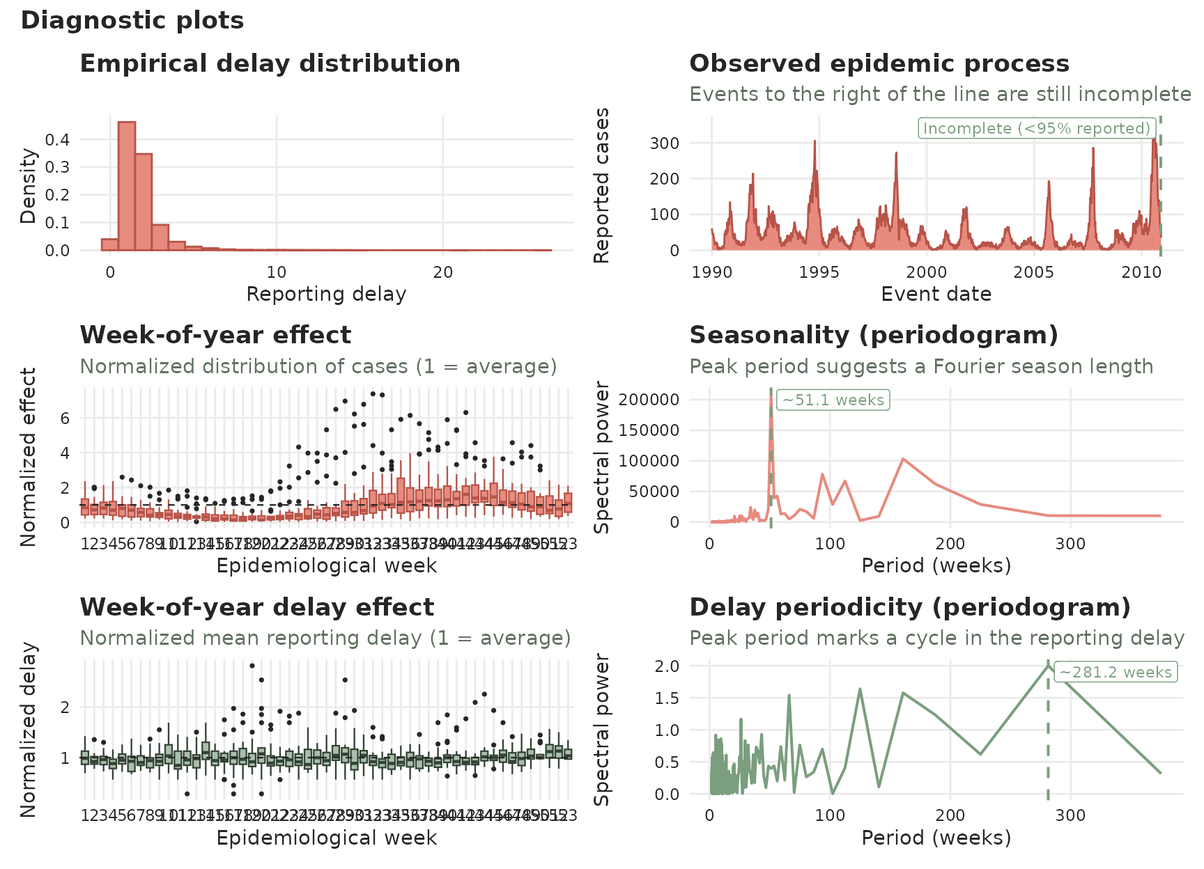
The autoplot() method gives a quick diagnostic overview of a tbl_now. Using ggplot2 and patchwork, it draws two families of panels. The case-count panels:

Empirical delay distribution: a case-count weighted histogram of the reporting delay.
Observed epidemic process: the latest reported counts per event_date.
Calendar effect: boxplots of the normalized effect (each event date’s cases divided by the overall mean, so 1 is average) by day of week / week of year / month.
Seasonality — a periodogram of the incidence series whose dominant peak suggests a Fourier season length to pass to temporal_effects().

…and the reporting-delay panels, which reveal delay effects (whether the delay itself has a calendar or periodic pattern):

Delay calendar effect: boxplots of the mean reporting delay by day of week / week of year / month.
Delay periodicity: a periodogram of the mean-delay series (e.g. a weekly reporting rhythm).

Which calendar/delay panels appear depends on the event unit (daily data gets day-of-week and week-of-year; weekly data week-of-year; monthly data month-of-year). Use the panels argument to pick a subset — for example panels = "delay_calendar" for just the delay boxplots, or a single key like panels = "delay_week" (a single panel is returned as a plain ggplot). The aliases are "all" (default), "calendar" and "delay_calendar".

Set by_strata = TRUE to split every panel by stratum: the boxplots become dodged boxes (one per stratum, side by side), the epidemic process and periodograms become one coloured line per stratum, and the delay distribution becomes dodged bars. The boxplots are then normalized per stratum (1 = that stratum’s own average) so the calendar pattern is comparable across strata. By default the object’s strata are used; pass strata = "gender" to group on a subset of the strata columns.

library(ggplot2)
library(patchwork)

dengue_now <- tbl_now(denguedat,
  event_date  = "onset_week",
  report_date = "report_week",
  verbose     = FALSE
)

autoplot(dengue_now)

For the weekly dengue data the periodogram peaks near 52 weeks, suggesting an annual cycle. We could capture this with a Fourier term of temporal_effects(seasons = 52).

Do delay distributions drift over time?

Reporting delays are not always stable: a surveillance system may speed up or slow down over a season or across years. plot_delay_drift() draws a rolling fan chart of the delay distribution indexed by event date — a solid rolling median, a dashed rolling mean, and 25–75% / 10–90% quantile bands. A rising or falling centre line signals location drift; widening or narrowing bands signal spread drift.

plot_delay_drift(dengue_now)

Because the most recent event dates have not had time to be fully reported, their delays look artificially short; that immature region (after the completeness cutoff) is shaded grey and should not be read as drift.

For a formal answer, test_delay_drift() runs an autocorrelation-robust monotonic-trend test (a modified Mann–Kendall test, via the modifiedmk package) on the per-period delay summaries — a delay series is correlated with itself, so an ordinary trend test would over-state significance. It tests both a location statistic (the median) and a dispersion statistic (the 10–90 spread), on mature data only:

test_delay_drift(dengue_now, stat = c("median", "spread"))
#> Warning: ! `test_delay_drift()` is experimental: results are not guaranteed and the
#>   interface may change.
#> ℹ Interpret a significant result as a potential trend change, not a confirmed
#>   one.
#> This warning is displayed once every 8 hours.
#> # A tibble: 2 × 9
#>   strata stat       n      tau sens_slope statistic p_value method    drift
#>   <chr>  <chr>  <int>    <dbl>      <dbl>     <dbl>   <dbl> <chr>     <lgl>
#> 1 all    median  1090 -0.00918          0    -0.243  0.808  hamed-rao FALSE
#> 2 all    spread  1090 -0.178            0    -2.32   0.0203 hamed-rao TRUE

A significant drift for spread with a non-significant one for median, say, would mean the typical delay held steady while its variability changed.

The trend test looks for gradual change. If instead you suspect an abrupt shift — a reporting-system change on some date — use test_delay_changepoint(), which applies Pettitt’s nonparametric change-point test and returns the estimated change date together with the before/after delay level:

test_delay_changepoint(dengue_now, stat = c("median", "spread"))
#> Warning: ! `test_delay_changepoint()` is experimental: results are not guaranteed and
#>   the interface may change.
#> ℹ Treat a detected change as a potential change point, not a confirmed one.
#> This warning is displayed once every 8 hours.
#> # A tibble: 2 × 10
#>   strata stat       n changepoint statistic  p_value before after  shift
#>   <chr>  <chr>  <int> <date>          <dbl>    <dbl>  <dbl> <dbl>  <dbl>
#> 1 all    median  1090 1998-01-19      38402 2.17e- 3   1.53  1.39 -0.136
#> 2 all    spread  1090 1997-09-01      93409 5.77e-18   2.55  1.91 -0.639
#> # ℹ 1 more variable: changepoint_detected <lgl>

You can mark the detected change point on the fan chart with plot_delay_drift(dengue_now, changepoint = TRUE).

Detecting batch reporting

Laboratories sometimes withhold results and then release a whole backlog at once — a batch. The key idea is that a batch moves reports along the report axis without creating them, so a window of report dates spanning both the lull and the spike has an unchanged total — whereas a genuine epidemic surge adds cases and inflates it. batch_screen() turns this into a per-report-date diagnostic that separates the two:

batches <- batch_screen(dengue_now, lookback = 2)

batches |>
  filter(batch) |>
  select(report_date, reported, baseline, deficit, delta, classification)
#> # A tibble: 69 × 6
#>    report_date reported baseline deficit    delta classification 
#>    <date>         <dbl>    <dbl>   <dbl>    <dbl> <chr>          
#>  1 1990-12-03       124     67    -44    101      batch_and_surge
#>  2 1991-02-04        53     38.4   14.5    0.0625 batch          
#>  3 1991-08-12        61     50.2   37.3  -26.6    batch          
#>  4 1991-12-02       241    154     12     75      batch_and_surge
#>  5 1992-01-20       126     99.2   50.0  -23.2    batch          
#>  6 1992-06-22        54     41.1   18.8   -5.83   batch          
#>  7 1993-01-18       150     62.2   -2.80  90.6    batch_and_surge
#>  8 1993-03-22        46     31.4   20.4   -5.73   batch          
#>  9 1993-09-27        65     40.7   21.5    2.85   batch          
#> 10 1993-10-25        83     53.4   24.7    4.88   batch          
#> # ℹ 59 more rows

The deficit (reports missing beforehand) is what flags a batch; delta (the window total minus its expected value) is what would flag a genuine surge. A volume spike alone is ambiguous — but a spike paid for by a preceding deficit, with delta near zero, is a batch. batch_shape_test() complements it by testing whether a flagged date drew on unusually old event dates. These functions are experimental; they are covered in depth, with the mathematics, in the Batch detection article.

Other functions (utilities)

Convert epidemiological weeks to dates

The function week_2_date() converts epidemiological week/year combinations into an aligned calendar date.

df <- data.frame(
  epidemiological_week = 1:5,
  epidemiological_year = rep(2024, 5)
)

df |>
  week_2_date(
    week_col = epidemiological_week,
    year_col = epidemiological_year
  )
#>   epidemiological_week epidemiological_year       date
#> 1                    1                 2024 2023-12-31
#> 2                    2                 2024 2024-01-07
#> 3                    3                 2024 2024-01-14
#> 4                    4                 2024 2024-01-21
#> 5                    5                 2024 2024-01-28

Reports

The functions get_initial_reported_cases() and get_latest_reported_cases() extract the number of cases first reported for each event date and the most recently reported totals, respectively. These utilities allow users to quantify revisions between initial and final reports.

df_reports <- data.frame(
  n = c(10, 1, 1, 0, 0, 3),
  event_date = rep(ymd("2020/09/12"), 6),
  report_date = c(
    ymd("2020/09/12"), ymd("2020/09/13"), ymd("2020/09/14"),
    ymd("2020/09/15"), ymd("2020/09/16"), ymd("2020/09/17")
  )
)

tbl_reports <- df_reports |>
  tbl_now(
    event_date = event_date, report_date = report_date,
    verbose = FALSE, case_count = n, report_units = "days",
    event_units = "days"
  )

tbl_reports
#> # A tibble:  6 × 6
#> # Data type: "count-incidence"
#> # Frequency: Event: `days` | Report: `days`
#>         n event_date   report_date   .event_num .report_num .delay
#>     <dbl> <date>       <date>             <dbl>       <dbl>  <dbl>
#>   [cases] [event_date] [report_date]      [...]       [...]  [...]
#> 1      10 2020-09-12   2020-09-12             0           0      0
#> 2       1 2020-09-12   2020-09-13             0           1      1
#> 3       1 2020-09-12   2020-09-14             0           2      2
#> 4       0 2020-09-12   2020-09-15             0           3      3
#> 5       0 2020-09-12   2020-09-16             0           4      4
#> 6       3 2020-09-12   2020-09-17             0           5      5
#> # ────────────────────────────────────────────────────────────────────────────────
#> # Now: 2020-09-17 | Event date: "event_date" | Report date: "report_date"
#> # ────────────────────────────────────────────────────────────────────────────────

The initial reported cases:

get_initial_reported_cases(tbl_reports)
#> # A tibble:  1 × 6
#> # Data type: "count-cumulative"
#> # Frequency: Event: `days` | Report: `days`
#>   event_date   report_date   .event_num .report_num       n .delay
#>   <date>       <date>             <dbl>       <dbl>   <dbl>  <dbl>
#>   [event_date] [report_date]      [...]       [...] [cases]  [...]
#> 1 2020-09-12   2020-09-12             0           0      10      0
#> # ────────────────────────────────────────────────────────────────────────────────
#> # Now: 2020-09-17 | Event date: "event_date" | Report date: "report_date"
#> # ────────────────────────────────────────────────────────────────────────────────

and the latest totals:

get_latest_reported_cases(tbl_reports)
#> # A tibble:  1 × 6
#> # Data type: "count-cumulative"
#> # Frequency: Event: `days` | Report: `days`
#>   event_date   report_date   .event_num .report_num       n .delay
#>   <date>       <date>             <dbl>       <dbl>   <dbl>  <dbl>
#>   [event_date] [report_date]      [...]       [...] [cases]  [...]
#> 1 2020-09-12   2020-09-17             0           5      15      5
#> # ────────────────────────────────────────────────────────────────────────────────
#> # Now: 2020-09-17 | Event date: "event_date" | Report date: "report_date"
#> # ────────────────────────────────────────────────────────────────────────────────

Week alignment

The align_weeks() function standardizes dates within the same epidemiological week to a single reference day (for example, the start of the week). This is helpful when computing differences across weekly reporting periods, avoiding fractional time intervals.

df <- data.frame(
  date = c(ymd("2022-10-31"), ymd("2022-11-07"), ymd("2022-11-13")),
  epiweek = c(44, 45, 46)
)

# Align to Sundays
df_aligned <- align_weeks(df, date_col = date)
df_aligned
#>         date epiweek date_aligned
#> 1 2022-10-31      44   2022-10-30
#> 2 2022-11-07      45   2022-11-06
#> 3 2022-11-13      46   2022-11-13

You can verify the resulting weekday using the wday() function from the lubridate package:

df_aligned |>
  mutate(day_label = wday(date_aligned, label = TRUE, abbr = FALSE))
#>         date epiweek date_aligned day_label
#> 1 2022-10-31      44   2022-10-30    Sunday
#> 2 2022-11-07      45   2022-11-06    Sunday
#> 3 2022-11-13      46   2022-11-13    Sunday

Complete zeroes

The complete_zeroes() function fills with zeroes those cases where the event or report weeks have not been observed.

Consider for example the following data with just two observations per date:

ndata <- tibble(
  event_date = c(as.Date("2021/01/12"), as.Date("2021/01/14"), as.Date("2021/01/14")),
  report_date = c(as.Date("2021/01/13"), as.Date("2021/01/15"), as.Date("2021/01/18")),
  case_count = c(10, 5, 1)
)

ndata <- tbl_now(ndata, event_date, report_date,
  verbose = FALSE, case_count = case_count, data_type = "count-incidence"
)

ndata
#> # A tibble:  3 × 6
#> # Data type: "count-incidence"
#> # Frequency: Event: `days` | Report: `days`
#>   event_date   report_date   case_count .event_num .report_num .delay
#>   <date>       <date>             <dbl>      <dbl>       <dbl>  <dbl>
#>   [event_date] [report_date]    [cases]      [...]       [...]  [...]
#> 1 2021-01-12   2021-01-13            10          0           1      1
#> 2 2021-01-14   2021-01-15             5          2           3      1
#> 3 2021-01-14   2021-01-18             1          2           6      4
#> # ────────────────────────────────────────────────────────────────────────────────
#> # Now: 2021-01-18 | Event date: "event_date" | Report date: "report_date"
#> # ────────────────────────────────────────────────────────────────────────────────

Notice that there are no observations for 2021/01/13. Furthermore, if we assume that the maximum possible observed delay is of 4, we can fill the unobserved cases with:

complete_zeroes(ndata, max_delay = 4)
#> # A tibble:  14 × 6
#> # Data type: "count-incidence"
#> # Frequency: Event: `days` | Report: `days`
#>    event_date   report_date   case_count .event_num .report_num .delay
#>    <date>       <date>             <dbl>      <int>       <dbl>  <dbl>
#>    [event_date] [report_date]    [cases]      [...]       [...]  [...]
#>  1 2021-01-12   2021-01-13            10          0           1      1
#>  2 2021-01-14   2021-01-15             5          2           3      1
#>  3 2021-01-12   2021-01-12             0          0           0      0
#>  4 2021-01-12   2021-01-14             0          0           2      2
#>  5 2021-01-12   2021-01-15             0          0           3      3
#>  6 2021-01-12   2021-01-16             0          0           4      4
#>  7 2021-01-13   2021-01-13             0          1           1      0
#>  8 2021-01-13   2021-01-14             0          1           2      1
#>  9 2021-01-13   2021-01-15             0          1           3      2
#> 10 2021-01-13   2021-01-16             0          1           4      3
#> 11 2021-01-13   2021-01-17             0          1           5      4
#> 12 2021-01-14   2021-01-14             0          2           2      0
#> 13 2021-01-14   2021-01-16             0          2           4      2
#> 14 2021-01-14   2021-01-17             0          2           5      3
#> # ────────────────────────────────────────────────────────────────────────────────
#> # Now: 2021-01-18 | Event date: "event_date" | Report date: "report_date"
#> # ────────────────────────────────────────────────────────────────────────────────

Which looks at all the possible report dates and event dates and sets the counts to zero if they have not been observed.

Censoring extreme delays

The function censor_delays_above() marks all delays above a threshold value (max_delay) as censored. This is useful to indicate extreme delays in some nowcast models:

df <- data.frame(
  onset = as.Date("2020-01-01") + c(0, 0, 1, 2),
  reported = as.Date("2020-01-01") + c(1, 5, 2, 300)
)
tn <- tbl_now(df,
  event_date = onset, report_date = reported,
  data_type = "linelist", verbose = FALSE
)

# the 300-day report becomes censored (an upper bound on its delay)
censor_delays_above(tn, max_delay = 60)
#> ℹ Marked 1 report with delay > 60 days as censored.
#> • This delay is now an upper bound (is_censored).
#> # A tibble:  4 × 6
#> # Data type: "linelist"
#> # Frequency: Event: `days` | Report: `days`
#>   onset        reported      .event_num .report_num .delay .is_censored 
#>   <date>       <date>             <dbl>       <dbl>  <dbl> <lgl>        
#>   [event_date] [report_date]      [...]       [...]  [...] [is_censored]
#> 1 2020-01-01   2020-01-02             0           1      1 FALSE        
#> 2 2020-01-01   2020-01-06             0           5      5 FALSE        
#> 3 2020-01-02   2020-01-03             1           2      1 FALSE        
#> 4 2020-01-03   2020-10-27             2         300    298 TRUE         
#> # ────────────────────────────────────────────────────────────────────────────────
#> # Now: 2020-10-27 | Event date: "onset" | Report date: "reported"
#> # Right-censored indicator: ".is_censored"
#> # ────────────────────────────────────────────────────────────────────────────────

Converting to data formats from other packages

NOTE This is still work in progress

tbl.now ships converters that move data between a tbl_now and the data structures used by other nowcasting and delay-estimation packages. They all follow the same naming convention:

tbl_now_from_*() builds a tbl_now (it wraps as_tbl_now(), so ... is forwarded to tbl_now()).
tbl_now_to_*() converts a tbl_now into that package’s native object.

Each function accepts a verbose argument that reports the choices it made (the inferred now, the data type, the units, the column mapping, and so on). The supported packages — epinowcast, baselinenowcast, EpiNow2, epidist, data.table and tsibble — are all optional (Suggests).

Package	`from`	`to`	Maps to
`epinowcast`	yes	yes	`count-cumulative` (`reference_date`, `report_date`, `confirm`); `from` also accepts a preprocessed `enw_preprocess_data` or fitted object
`baselinenowcast`	yes	yes	`count-incidence` (long data frame or reporting-triangle matrix)
`EpiNow2`	—	yes	a single `date`/`confirm` series for `estimate_infections()`, or (with `model = "estimate_truncation"`) a list of report-date snapshots for `estimate_truncation()`
`data.table`	yes	yes	any data type
`epidist`	yes	yes	`linelist` (primary/secondary event dates)
`tsibble`	yes	yes	a `tbl_ts` (one date as index, the other date + strata as key)

The object produced by any tbl_now_to_*() can be converted straight back with as_tbl_now(), which has methods for each of these classes:

dengue_now <- tbl_now(denguedat,
  event_date = "onset_week",
  report_date = "report_week", strata = "gender",
  verbose = FALSE
)

# tbl_now -> tsibble -> tbl_now
dengue_ts <- tbl_now_to_tsibble(dengue_now, verbose = FALSE)
#> Warning: tsibble requires unique index/key rows; aggregating linelist to
#> "count-incidence" with `to_count()`.
as_tbl_now(dengue_ts, report_date = "report_week", verbose = FALSE)
#> # A tibble:  8,265 × 7
#> # Data type: "linelist"
#> # Frequency: Event: `weeks` | Report: `weeks`
#>    onset_week   report_week   gender       n .event_num .report_num .delay
#>    <date>       <date>        <chr>    <int>      <dbl>       <dbl>  <dbl>
#>    [event_date] [report_date] [strata] [...]      [...]       [...]  [...]
#>  1 1990-01-01   1990-01-01    Female       2          0           0      0
#>  2 1990-01-01   1990-01-01    Male         1          0           0      0
#>  3 1990-01-01   1990-01-08    Female      13          0           1      1
#>  4 1990-01-08   1990-01-08    Female       1          1           1      0
#>  5 1990-01-01   1990-01-08    Male        11          0           1      1
#>  6 1990-01-08   1990-01-08    Male         1          1           1      0
#>  7 1990-01-01   1990-01-15    Female      16          0           2      2
#>  8 1990-01-08   1990-01-15    Female      17          1           2      1
#>  9 1990-01-15   1990-01-15    Female       2          2           2      0
#> 10 1990-01-01   1990-01-15    Male         7          0           2      2
#> # ────────────────────────────────────────────────────────────────────────────────
#> # Now: 2010-12-20 | Event date: "onset_week" | Report date: "report_week"
#> # Strata: "gender"
#> # ────────────────────────────────────────────────────────────────────────────────
#> # ℹ 8,255 more rows

For example, the epinowcast hospitalization data ships in long cumulative format and converts straight into a count-cumulative tbl_now:

library(epinowcast)
data(germany_covid19_hosp)


#Read data from epinowcast
obs  <- germany_covid19_hosp[location == "DE"]

#Remove unused column
obs  <- obs[, location := NULL]

#Pre-process data
pobs <- epinowcast::enw_preprocess_data(obs, max_delay = 40, by = "age_group")

hospitalizations_now <- tbl_now_from_epinowcast(pobs)
  
hospitalizations_now
#> # A tibble:  48,279 × 7
#> # Data type: "count-cumulative"
#> # Frequency: Event: `days` | Report: `days`
#>    reference_date report_date   confirm age_group .event_num .report_num .delay
#>    <date>         <date>          <int> <fct>          <dbl>       <dbl>  <dbl>
#>    [event_date]   [report_date] [cases] [strata]       [...]       [...]  [...]
#>  1 2021-04-06     2021-04-06        149 00+                0           0      0
#>  2 2021-04-06     2021-04-07        289 00+                0           1      1
#>  3 2021-04-06     2021-04-08        350 00+                0           2      2
#>  4 2021-04-06     2021-04-09        402 00+                0           3      3
#>  5 2021-04-06     2021-04-10        438 00+                0           4      4
#>  6 2021-04-06     2021-04-11        446 00+                0           5      5
#>  7 2021-04-06     2021-04-12        456 00+                0           6      6
#>  8 2021-04-06     2021-04-13        468 00+                0           7      7
#>  9 2021-04-06     2021-04-14        493 00+                0           8      8
#> 10 2021-04-06     2021-04-15        508 00+                0           9      9
#> # ────────────────────────────────────────────────────────────────────────────────
#> # Now: 2021-10-20 | Event date: "reference_date" | Report date: "report_date"
#> # Strata: "age_group"
#> # ────────────────────────────────────────────────────────────────────────────────
#> # ℹ 48,269 more rows

Going the other way, tbl_now_to_epinowcast() returns an enw_preprocess_data object ready for epinowcast::epinowcast():

epinowcast_object <- tbl_now_to_epinowcast(hospitalizations_now, verbose = FALSE)
#> Warning: ! Converting a <tbl_now> to epinowcast is lossy: the result is not guaranteed
#>   to be identical to a native epinowcast object.
#> ℹ Some information might be dropped (e.g. covariate columns, maximum delays,
#>   grouping indices and padding rows).
#> ℹ If you have the original data as a `tibble`, `data.frame` or `data.table`,
#>   prefer using that directly over converting from another format.
#> ℹ Silence this warning with `quiet = TRUE`.
epinowcast_object
#> ── Preprocessed nowcast data ─────────────────────────────────────────────────── 
#> Groups: 7 (age_group) | Timestep: day | Max delay: 40 
#> Observations: 198 timepoints x 1386 snapshots 
#> Max date: 2021-10-20 
#> 
#> Datasets (access with `enw_get_data(x, "<name>")`): 
#>   obs                :  49,980 x 8 
#>   new_confirm        :  49,980 x 10 
#>   latest             :   1,386 x 9 
#>   missing_reference  :       0 x 5 
#>   reporting_triangle :   1,386 x 42 
#>   metareference      :   1,386 x 8 
#>   metareport         :   1,659 x 11 
#>   metadelay          :      40 x 5

The same pattern works for the other packages.

References

Dancho, Matt, and Davis Vaughan. 2023. Timetk: A Tool Kit for Working with Time Series. https://doi.org/10.32614/CRAN.package.timetk.

Gelman, Andrew, Aki Vehtari, Daniel Simpson, et al. 2020. “Bayesian Workflow.” arXiv Preprint arXiv:2011.01808.

Wang, Earo, Dianne Cook, and Rob J Hyndman. 2020. “A New Tidy Data Structure to Support Exploration and Modeling of Temporal Data.” Journal of Computational and Graphical Statistics 29 (3): 466–78.

Wang, Yiru. 2019. “Tidy Tools for Supporting Fluent Workflow in Temporal Data Analysis.” PhD thesis, Monash University.

Wickham, Hadley. 2014. “Tidy Data.” Journal of Statistical Software 59: 1–23.

Wickham, Hadley, Mara Averick, Jennifer Bryan, et al. 2019. “Welcome to the tidyverse.” Journal of Open Source Software 4 (43): 1686. https://doi.org/10.21105/joss.01686.

Wickham, Hadley, Mine Çetinkaya-Rundel, and Garrett Grolemund. 2023. R for Data Science: Import, Tidy, Transform, Visualize, and Model Data. O’Reilly Media, Inc.

The tbl.now Framework

Example

Attributes of a tbl_now()

Data types

Converting Between Data Types

Temporal effects

Lazy evaluation: attach first, compute later

After-holiday and after-weekend effects

Event- vs report-date effects

Modifying a tbl_now() with dplyr

Modifying a tbl_now() with dplyr

Updating a tbl_now()

Visualizing a tbl_now

Do delay distributions drift over time?

Detecting batch reporting

Other functions (utilities)

Convert epidemiological weeks to dates

Reports

Week alignment

Complete zeroes

Censoring extreme delays

Converting to data formats from other packages

References

The `tbl.now` Framework

Modifying a tbl_now() with `dplyr`

Visualizing a `tbl_now`