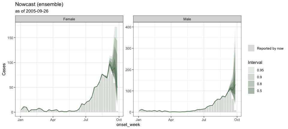
tbl.now provides an extension of the tibble() for storing, validating, and manipulating epidemiological nowcasting data. It standardizes the representation of event dates, report dates, strata, temporal covariates, and data types (linelist and cumulative), ensuring that downstream models within the diseasenowcasting ecosystem can rely on a consistent interface.
Installation
Install the development version from GitHub:
# install.packages("pak") # <- uncomment if you do not have `pak`
pak::pkg_install("RodrigoZepeda/tbl.now")Load the package:
A minimal example
Suppose you have a dataset where n cases reported on report_date belong to events occurring on event_date:
df <- tibble(
event_date = c(
ymd("2023-12-25"), ymd("2023-12-26"),
ymd("2023-12-25"), ymd("2023-12-26")
),
report_date = c(
ymd("2023-12-26"), ymd("2023-12-26"),
ymd("2023-12-27"), ymd("2023-12-27")
),
n = c(10, 2, 5, 11)
)Convert it to a tbl_now():
df_now <- df |>
tbl_now(event_date = event_date, report_date = report_date, case_count = n)
#> ℹ Identified data as <count-incidence> with counts in column "n".
df_now
#> # A tibble: 4 × 6
#> # Data type: "count-incidence"
#> # Frequency: Event: `days` | Report: `days`
#> event_date report_date n .event_num .report_num .delay
#> <date> <date> <dbl> <dbl> <dbl> <dbl>
#> [event_date] [report_date] [cases] [...] [...] [...]
#> 1 2023-12-25 2023-12-26 10 0 1 1
#> 2 2023-12-26 2023-12-26 2 1 1 0
#> 3 2023-12-25 2023-12-27 5 0 2 2
#> 4 2023-12-26 2023-12-27 11 1 2 1
#> # ────────────────────────────────────────────────────────────────────────────────
#> # Now: 2023-12-27 | Event date: "event_date" | Report date: "report_date"
#> # ────────────────────────────────────────────────────────────────────────────────tbl_now() automatically:
infers that the data type is linelist (one row per event)
determines the date units (daily event and report frequencies)
computes numerical versions of the dates:
.event_num,.report_num, and.delaysets the now to the most recent reporting date
Use it like any tibble:
df_now |>
filter(n > 5)
#> # A tibble: 2 × 6
#> # Data type: "count-incidence"
#> # Frequency: Event: `days` | Report: `days`
#> event_date report_date n .event_num .report_num .delay
#> <date> <date> <dbl> <dbl> <dbl> <dbl>
#> [event_date] [report_date] [cases] [...] [...] [...]
#> 1 2023-12-25 2023-12-26 10 0 1 1
#> 2 2023-12-26 2023-12-27 11 1 2 1
#> # ────────────────────────────────────────────────────────────────────────────────
#> # Now: 2023-12-27 | Event date: "event_date" | Report date: "report_date"
#> # ────────────────────────────────────────────────────────────────────────────────Note Linelist, count-incidence and count-cumulative data is available for a
tbl_now. See the data types section oftbl_now()for more information.
Adding strata
If strata was given, the tbl_now() can easily tag the corresponding strata.
# Add the column using dplyr:
df_now <- df_now |>
mutate(sex = c("M", "M", "F", "M"))
df_now
#> # A tibble: 4 × 7
#> # Data type: "count-incidence"
#> # Frequency: Event: `days` | Report: `days`
#> event_date report_date n .event_num .report_num .delay sex
#> <date> <date> <dbl> <dbl> <dbl> <dbl> <chr>
#> [event_date] [report_date] [cases] [...] [...] [...] [...]
#> 1 2023-12-25 2023-12-26 10 0 1 1 M
#> 2 2023-12-26 2023-12-26 2 1 1 0 M
#> 3 2023-12-25 2023-12-27 5 0 2 2 F
#> 4 2023-12-26 2023-12-27 11 1 2 1 M
#> # ────────────────────────────────────────────────────────────────────────────────
#> # Now: 2023-12-27 | Event date: "event_date" | Report date: "report_date"
#> # ────────────────────────────────────────────────────────────────────────────────Use the add_strata to specify the new column is a stratum:
df_now |>
add_strata("sex")
#> # A tibble: 4 × 7
#> # Data type: "count-incidence"
#> # Frequency: Event: `days` | Report: `days`
#> event_date report_date n .event_num .report_num .delay sex
#> <date> <date> <dbl> <dbl> <dbl> <dbl> <chr>
#> [event_date] [report_date] [cases] [...] [...] [...] [strata]
#> 1 2023-12-25 2023-12-26 10 0 1 1 M
#> 2 2023-12-26 2023-12-26 2 1 1 0 M
#> 3 2023-12-25 2023-12-27 5 0 2 2 F
#> 4 2023-12-26 2023-12-27 11 1 2 1 M
#> # ────────────────────────────────────────────────────────────────────────────────
#> # Now: 2023-12-27 | Event date: "event_date" | Report date: "report_date"
#> # Strata: "sex"
#> # ────────────────────────────────────────────────────────────────────────────────The object now records "sex" as a stratification variable, preserved through downstream operations.
Adding temporal effects
Temporal covariates help nowcasting models incorporate weekly seasonality, holiday effects, etc. Define the effects:
t_eff <- temporal_effects(
day_of_week = TRUE,
week_of_year = TRUE,
holidays = cal_us_federal()
)
t_eff
#>
#> ── Temporal Effects ────────────────────────────────────────────────────────────
#> The following effects are in place:
#> • "day_of_week"
#> • "week_of_year"
#> • "holidays":
#> 1. New Year's Day, US Martin Luther King Jr. Day, US Presidents' Day, US
#> Memorial Day, US Juneteenth, US Independence Day, US Labor Day, US Indigenous
#> Peoples' Day, US Veterans Day, US Thanksgiving, and ChristmasAttach them to the dataset:
df_now <- df_now |>
add_temporal_effects(t_eff)
df_now
#> # A tibble: 4 × 7
#> # Data type: "count-incidence"
#> # Frequency: Event: `days` | Report: `days`
#> event_date report_date n .event_num .report_num .delay sex
#> <date> <date> <dbl> <dbl> <dbl> <dbl> <chr>
#> [event_date] [report_date] [cases] [...] [...] [...] [...]
#> 1 2023-12-25 2023-12-26 10 0 1 1 M
#> 2 2023-12-26 2023-12-26 2 1 1 0 M
#> 3 2023-12-25 2023-12-27 5 0 2 2 F
#> 4 2023-12-26 2023-12-27 11 1 2 1 M
#> # ────────────────────────────────────────────────────────────────────────────────
#> # Now: 2023-12-27 | Event date: "event_date" | Report date: "report_date"
#> # T. effects (lazy): [event_date] day_of_week, week_of_year, holidays
#> # ────────────────────────────────────────────────────────────────────────────────This lazily adds to the table day_of_week, week_of_year, and holiday related to event_date. However it does not compute. Use compute_temporal_effects() to add them as columns:
df_now |>
compute_temporal_effects()
#> # A tibble: 4 × 10
#> # Data type: "count-incidence"
#> # Frequency: Event: `days` | Report: `days`
#> event_date report_date n .event_num .report_num .delay sex
#> <date> <date> <dbl> <dbl> <dbl> <dbl> <chr>
#> [event_date] [report_date] [cases] [...] [...] [...] [...]
#> 1 2023-12-25 2023-12-26 10 0 1 1 M
#> 2 2023-12-26 2023-12-26 2 1 1 0 M
#> 3 2023-12-25 2023-12-27 5 0 2 2 F
#> 4 2023-12-26 2023-12-27 11 1 2 1 M
#> .event_day_of_week .event_week_of_year .event_holiday
#> <int> <int> <int>
#> [t_effect] [t_effect] [t_effect]
#> 1 2 1 1
#> 2 3 1 0
#> 3 2 1 1
#> 4 3 1 0
#> # ────────────────────────────────────────────────────────────────────────────────
#> # Now: 2023-12-27 | Event date: "event_date" | Report date: "report_date"
#> # T. effects: [event_date] day_of_week, week_of_year, holidays
#> # T. effect cols: ".event_day_of_week", ".event_week_of_year", and
#> # ".event_holiday"
#> # ────────────────────────────────────────────────────────────────────────────────You can also attach effects related to the report_date:
r_eff <- temporal_effects(day_of_week = TRUE)
df_now |>
add_temporal_effects(r_eff, date_type = "report_date")
#> # A tibble: 4 × 7
#> # Data type: "count-incidence"
#> # Frequency: Event: `days` | Report: `days`
#> event_date report_date n .event_num .report_num .delay sex
#> <date> <date> <dbl> <dbl> <dbl> <dbl> <chr>
#> [event_date] [report_date] [cases] [...] [...] [...] [...]
#> 1 2023-12-25 2023-12-26 10 0 1 1 M
#> 2 2023-12-26 2023-12-26 2 1 1 0 M
#> 3 2023-12-25 2023-12-27 5 0 2 2 F
#> 4 2023-12-26 2023-12-27 11 1 2 1 M
#> # ────────────────────────────────────────────────────────────────────────────────
#> # Now: 2023-12-27 | Event date: "event_date" | Report date: "report_date"
#> # T. effects (lazy): [event_date] day_of_week, week_of_year, holidays |
#> # [report_date] day_of_week
#> # ────────────────────────────────────────────────────────────────────────────────Working with the “now”
You may override the default now to perform historical evaluation:
df_pruned <- df_now |>
filter(report_date <= ymd("2023-12-26")) |>
change_now(ymd("2023-12-26"))Retrieve the current active nowcast horizon:
get_now(df_pruned)
#> [1] "2023-12-26"Visualizing a tbl_now
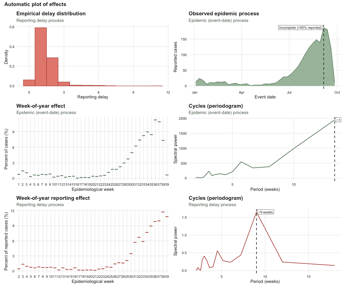
The autoplot() method gives a quick diagnostic overview of a tbl_now.
library(ggplot2)
library(patchwork)
data("mpoxdat")
mpoxdat_now <- tbl_now(mpoxdat,
event_date = dx_date,
report_date = dx_report_date,
case_count = n,
verbose = FALSE
)
autoplot(mpoxdat_now)
Diagnosing reporting problems
tbl.now also diagnoses common reporting artefacts directly from the data.
Does the reporting delay drift over time?
The plot_delay_drift() function draws a rolling fan chart of the delay distribution, while test_delay_drift() and test_delay_changepoint() test for a gradual trend or an abrupt change.
data("covid_colombia")
covidat_now <- covid_colombia %>%
filter(notification_date <= as.Date("2021/01/01"),
diagnosis_date <= as.Date("2021/01/01")) %>%
tbl_now(
event_date = notification_date,
report_date = diagnosis_date,
case_count = n,
strata = sex,
verbose = FALSE,
data_type = "count-incidence"
)
plot_delay_drift(covidat_now, changepoint = TRUE)
We can see that the delay does change in time varying a lot at the beginning of the epidemic (before April) then stabilizing between April and July, and finally shifting downwards around August. The changepoint option uses Pettitt’s test to identify one changepoint in the data. It can be recovered with test_delay_changepoint():
test_delay_changepoint(covidat_now)
#> Warning: ! `test_delay_changepoint()` is experimental: results are not guaranteed and
#> the interface may change.
#> ℹ Treat a detected change as a potential change point, not a confirmed one.
#> This warning is displayed once every 8 hours.
#> # A tibble: 2 × 10
#> strata stat n changepoint statistic p_value before after shift
#> <chr> <chr> <int> <date> <dbl> <dbl> <dbl> <dbl> <dbl>
#> 1 all median 292 2020-08-17 11818 5.41e-15 5.90 3.92 -1.98
#> 2 all spread 292 2020-05-09 8670 2.89e- 8 8.85 11.1 2.25
#> changepoint_detected
#> <lgl>
#> 1 TRUE
#> 2 TRUEAs context, on August 10th 2020 the Colombian government anounced the massive use of antigen testing for COVID-19 and in August 25th implemented the PRASS programme]which shifted the sampling and reporting paradigm for the country (Osorio Saldarriga et al). These are the changes potentially identified by test_delay_changepoint().
[!NOTE] Pettitt’s test in
test_delay_changepoint()detects only one change point: the largest one. If your data has more than one changepoint break your data into chuncks and run the test for each of them.
Batch reporting
Some systems might withhold results and then release their backlog at once. Such batches displace reports along the report axis by first not presenting them in time and then reporting all in bulk. Batches do not create new cases they just shift their report dates to a later period.
The batch_test() function uses this idea to identify batches. The confidence level can be set with alpha. For example here we set a level of 80%:
covidat_now %>%
remove_all_strata() %>%
batch_test(period = 7, alpha = 0.2) #> # A tibble: 302 × 9
#> report_date reported baseline p_transport_bh batch stratum deficit delta
#> <date> <dbl> <dbl> <dbl> <lgl> <chr> <dbl> <dbl>
#> 1 2020-07-19 7880 5273. 0.179 TRUE all 2806. -199.
#> 2 2020-10-02 9713 7908. 0.159 TRUE all 3042. -1237.
#> 3 2020-11-20 11259 8655. 0.108 TRUE all 3636. -1032.
#> 4 2020-03-06 1 NA NA FALSE all NA NA
#> 5 2020-03-07 0 NA NA FALSE all NA NA
#> 6 2020-03-08 0 NA NA FALSE all NA NA
#> 7 2020-03-09 2 NA NA FALSE all NA NA
#> 8 2020-03-10 0 NA NA FALSE all NA NA
#> 9 2020-03-11 6 NA NA FALSE all NA NA
#> 10 2020-03-12 4 NA NA FALSE all NA NA
#> p_transport
#> <dbl>
#> 1 0.0508
#> 2 0.0437
#> 3 0.0265
#> 4 NA
#> 5 NA
#> 6 NA
#> 7 NA
#> 8 NA
#> 9 NA
#> 10 NA
#> # ℹ 292 more rowsAdditional batch detection tools can be found in the corresponding article.
Extreme delays
Extreme delays can be censored with the censor_delays_above() function that assigns upper bounds to the delay. In the following data frame for example, an extreme delay of 300 is marked as censored with that function:
df <- data.frame(
onset = as.Date("2020-01-01") + c(0, 0, 1, 2),
reported = as.Date("2020-01-01") + c(1, 5, 2, 300)
)
tn <- tbl_now(df,
event_date = onset, report_date = reported,
data_type = "linelist", verbose = FALSE
)
# the 300-day report becomes censored (an upper bound on its delay)
censor_delays_above(tn, max_delay = 60)
#> ℹ Marked 1 report with delay > 60 days as censored.
#> • This delay is now an upper bound (is_censored).
#> # A tibble: 4 × 6
#> # Data type: "linelist"
#> # Frequency: Event: `days` | Report: `days`
#> onset reported .event_num .report_num .delay .is_censored
#> <date> <date> <dbl> <dbl> <dbl> <lgl>
#> [event_date] [report_date] [...] [...] [...] [is_censored]
#> 1 2020-01-01 2020-01-02 0 1 1 FALSE
#> 2 2020-01-01 2020-01-06 0 5 5 FALSE
#> 3 2020-01-02 2020-01-03 1 2 1 FALSE
#> 4 2020-01-03 2020-10-27 2 300 298 TRUE
#> # ────────────────────────────────────────────────────────────────────────────────
#> # Now: 2020-10-27 | Event date: "onset" | Report date: "reported"
#> # Right-censored indicator: ".is_censored"
#> # ────────────────────────────────────────────────────────────────────────────────Learning more
- Introduction vignette: https://rodrigozepeda.github.io/tbl.now/articles/tbl.now.html
- Full walk-through with real CDC Flusight data: https://rodrigozepeda.github.io/tbl.now/articles/Example.html
- Tutorial on detecting batches and other reporting-delay artifacts: https://rodrigozepeda.github.io/tbl.now/articles/batch-reporting.html
- Package reference: https://rodrigozepeda.github.io/tbl.now/reference/