Using tbl.now with different modelling packages

Why this vignette?

Preparing the same data different ways for the different nowcasting models can be tedious and error-prone. This is exactly what tbl.now helps with. You can describe your data once by specifying which column is the event_date, which is the report_date, whether your data is linelist or has counts (and what those counts mean!) and tbl.now will hand it to each modelling package in the format that package expects.

In this vignette we take a single dataset (covid_colombia), and from that one object, use several different nowcasting / delay-estimation tools:

Package	What it does	Additional requirements	`tbl.now` converter	`run_nowcast()` method
diseasenowcasting	flexible Bayesian nowcast (delay + epidemic processes)	none (uses `RTMB`)	consumes a `tbl_now` directly	`"diseasenowcasting"`
baselinenowcast	fast, assumption-light baseline nowcast	none	`tbl_now_to_baselinenowcast()`	`"baselinenowcast"`
epinowcast	flexible Bayesian nowcast (delay + reference modules)	Stan	`tbl_now_to_epinowcast()`	`"epinowcast"`
epidist	estimates only the reporting delay distribution	Stan	`tbl_now_to_epidist()`	— (not a nowcast)
NobBS	Nowcasting by Bayesian Smoothing	JAGS	`tbl_now_to_nobbs()`	`"NobBS"`
surveillance	the classic Höhle & an der Heiden nowcast	none for the method used here (JAGS for `bayes.trunc.ddcp`)	`tbl_now_to_surveillance()`	`"surveillance"`
EpiNow2	renewal-equation R_t, reporting truncation, and delay distributions	Stan (`cmdstanr`)	`tbl_now_to_EpiNow2()`	`"EpiNow2"`

You do not need to be an expert in any of these packages. The point of this vignette is to show you how to use any of them for nowcasting.

This article shows you to to use each package individually. The tbl.now package contains the run_nowcast() function which allows you run nowcast models without requiring knowledge of each of the package’s frameworks. We recommend reading the article One call, many models first if your priority is to do nowcasts. Read this one if your prioirity is understanding how to use tbl.now for a specific package. In that case, read the description on The data and then go to your favourite package’s section.

This article solely aims to show how to use tbl.now within each package’s own framework. We are purposefully not using or searching for the most optimal models from each package. Please DO NOT CONCLUDE WHICH PACKAGE IS BEST BASED ON THE RESULTS FROM THIS TUTORIAL.

The data

tbl.now includes covid_colombia, daily COVID-19 case counts from Colombia’s national surveillance system (INS) from 2020 to 2023. Each row is a (notification_date, diagnosis_date, sex) combination with a case count n. It includes notification date as the date the case was first notified (event_date), and the date the laboratory diagnosis was registered (report_date). The gap between the two is the reporting delay.

OUR GOAL IS TO NOWCAST THE CASES AS THEY HAPPEN ACCORDING TO notification_date.

library(dplyr)
library(lubridate)
library(tbl.now)

data(covid_colombia)

#>   notification_date diagnosis_date    sex n
#> 1        2020-03-02     2020-03-06 Female 1
#> 2        2020-03-03     2020-03-14 Female 1
#> 3        2020-03-06     2020-03-09   Male 1
#> 4        2020-03-07     2020-03-09 Female 1
#> 5        2020-03-08     2020-03-11 Female 2
#> 6        2020-03-09     2020-03-11 Female 1

We will build a single tbl_now. To do so, we state which column is the event date (notification_date), which is the report date (diagnosis_date), and which the counts (n); tbl.now infers the rest: that the grid is daily, and that the “now” is the last report date.

For this example we will cut both dates at the start of April 2021 (Colombia’s third wave). The example will assume we are back on that date, with only the information available until then (now = "2021-04-01"). No data observed after that date is kept:

#Filter to simulate being back on April 2021
covid <- covid_colombia |>
  filter(notification_date < as.Date("2021-04-01") & 
           diagnosis_date < as.Date("2021-04-01"))

#Create the tbl_now object
covid_now <- covid |>
  tbl_now(
    event_date  = notification_date,
    report_date = diagnosis_date,
    case_count  = n,
    data_type   = "count-incidence"
  )
#> Warning: *Non-unique*: 8066 rows share a (notification_date, diagnosis_date) combination.
#> ℹ 1 column "sex" is not declared, so it splits each cell into several rows. Declare it with `strata = ` to model it separately, or `to_count()` to pool it
#>   away. The `tbl_now_to_()` converters pool undeclared columns for you, so this is a warning rather than an error.

#We can see the tbl_now
covid_now
#> # A tibble:  18,195 × 7
#> # Data type: "count-incidence"
#> # Frequency: Event: `days` | Report: `days`
#>   notification_date diagnosis_date sex          n .event_num .report_num .delay
#>   <date>            <date>         <chr>    <int>      <dbl>       <dbl>  <dbl>
#>   [event_date]      [report_date]  [...]  [cases]      [...]       [...]  [...]
#> 1 2020-03-02        2020-03-06     Female       1          0           4      4
#> 2 2020-03-03        2020-03-14     Female       1          1          12     11
#> 3 2020-03-06        2020-03-09     Male         1          4           7      3
#> 4 2020-03-07        2020-03-09     Female       1          5           7      2
#> 5 2020-03-08        2020-03-11     Female       2          6           9      3
#> # ────────────────────────────────────────────────────────────────────────────────────────────────────────────────────────────────────────────────────────────────
#> # Now: 2021-03-31 | Event date: "notification_date" | Report date: "diagnosis_date"
#> # ────────────────────────────────────────────────────────────────────────────────────────────────────────────────────────────────────────────────────────────────
#> # ℹ 18,190 more rows

About the warning. sex is in the data but was not declared as a covariate or strata, so each (notification_date, diagnosis_date) cell has two rows (one per sex). One can correct it by summing the (notification_date, diagnosis_date) combinations by sex with to_count():

covid_now |> 
  to_count(to = "count-incidence")

Though for the purpose of this tutorial we will ignore the warning. That is because we will also create a second tbl.now from this one. The new one will be stratified by sex to show how the related packages work both in the stratified and not stratified case.

Everything in this article is built from either this dataset or a more complete one with strata and temporal effects.

A more complex object: strata and temporal effects

Reporting delays are rarely constant and many series are reported for several strata (here, sex) that you may want to nowcast separately. Here we build a second object, covid_seasonal, that declares sex as a stratum and adds day-of-week plus annual-Fourier temporal (delay) effects. We show how one would use them after converting to each package’s format:

covid_seasonal <- covid_now |> 
  add_strata(sex) |> 
  add_temporal_effects(
    temporal_effects(
      day_of_week = TRUE,    # a separate level per weekday
      seasons     = 365      # an annual Fourier cycle (period = 365 days)
    )
  )

A note on series length. This dataset carries 2.35 million cases. And not all packages will be able to handle that amount of data. Specifically we will see that:

diseasenowcasting can take the whole series.
baselinenowcast can keep every event day, but the delays will be capped with max_delay = 30 (the real maximum delay in the data corresponds to 185 days).
The remaining packages (NobBS, surveillance, epinowcast and epidist) will be trimmed both in the number of events and delays as the time it takes
to run those models is prohibitively expensive.

diseasenowcasting

Install with:

install.packages("diseasenowcasting", repos = c("https://rodrigozepeda.r-universe.dev", getOption("repos")))

diseasenowcasting is designed hand-in-hand with tbl.now, so it takes a tbl_now directly. You just hand it the object:

Simple nowcast

library(diseasenowcasting)
dnc_fit <- nowcast(covid_now)

dnc_fit

#> ── A <tbl_nowcast> from method "diseasenowcasting" ─────────────────────────────────────────────────────────────────────────────────────────────
#> • now: "2021-03-31"
#> • event dates: 395
#> • quantile levels: 0.025, 0.05, 0.1, 0.25, 0.5, 0.75, 0.9, 0.95, and 0.975
#> • draws: 2000
#> 
#> Nowcast at "2021-03-31" (q50, 2.5-97.5% interval):
#> • 11,561 [8,126.4, 18,426.7]
#> 
#> # A tibble: 6 × 3
#>   notification_date .quantile_level .value
#>   <date>                      <dbl>  <dbl>
#> 1 2020-03-02                  0.025      1
#> 2 2020-03-02                  0.05       1
#> 3 2020-03-02                  0.1        1
#> 4 2020-03-02                  0.25       1
#> 5 2020-03-02                  0.5        1
#> # ℹ 1 more row
#> ℹ 3549 more rows. Use `as_tibble()` for all of them.

Predictions can be obtained via tidy:

tidy(dnc_fit)

#> # A tibble: 5 × 7
#>   event_date stratum estimate conf.low conf.high level engine           
#>   <date>     <chr>      <dbl>    <dbl>     <dbl> <dbl> <chr>            
#> 1 2021-03-27 all        7929     6690.    10604.  0.95 diseasenowcasting
#> 2 2021-03-28 all        5761     4435.     8763.  0.95 diseasenowcasting
#> 3 2021-03-29 all       11040     9230.    14911.  0.95 diseasenowcasting
#> 4 2021-03-30 all       11328.    8748.    16218.  0.95 diseasenowcasting
#> 5 2021-03-31 all       11561     8126.    18427.  0.95 diseasenowcasting

With strata and effects.

diseasenowcasting reaches into the tbl_now itself, so the enriched object needs no extra arguments: it picks up the sex stratum and the day-of-week / seasonal effect columns automatically.

dnc_seasonal <- nowcast(covid_seasonal)   # strata and effects used automatically

#> ── A <tbl_nowcast> from method "diseasenowcasting" ─────────────────────────────────────────────────────────────────────────────────────────────
#> • now: "2021-03-31"
#> • event dates: 395
#> • strata: "sex"
#> • quantile levels: 0.025, 0.05, 0.1, 0.25, 0.5, 0.75, 0.9, 0.95, and 0.975
#> • draws: 2000
#> 
#> Nowcast at "2021-03-31" (q50, 2.5-97.5% interval):
#> • Female: 6,442.5 [4,551.9, 9,868.1]
#> • Male: 5,738.5 [3,962.9, 8,822.3]
#> 
#> # A tibble: 6 × 4
#>   notification_date sex    .quantile_level .value
#>   <date>            <chr>            <dbl>  <dbl>
#> 1 2020-03-02        Female           0.025      1
#> 2 2020-03-02        Female           0.05       1
#> 3 2020-03-02        Female           0.1        1
#> 4 2020-03-02        Female           0.25       1
#> 5 2020-03-02        Female           0.5        1
#> # ℹ 1 more row
#> ℹ 7104 more rows. Use `as_tibble()` for all of them.

tidy() can also be used in stratified cases:

tidy(dnc_seasonal)

#> # A tibble: 5 × 7
#>   event_date stratum estimate conf.low conf.high level engine           
#>   <date>     <chr>      <dbl>    <dbl>     <dbl> <dbl> <chr>            
#> 1 2021-03-27 Male       3724     3079.     4867.  0.95 diseasenowcasting
#> 2 2021-03-28 Male       2848.    2152      4266.  0.95 diseasenowcasting
#> 3 2021-03-29 Male       5347     4416.     7116.  0.95 diseasenowcasting
#> 4 2021-03-30 Male       5476.    4215.     7736.  0.95 diseasenowcasting
#> 5 2021-03-31 Male       5738.    3963.     8822.  0.95 diseasenowcasting

Three panels (Total, Female, Male) comparing the diseasenowcasting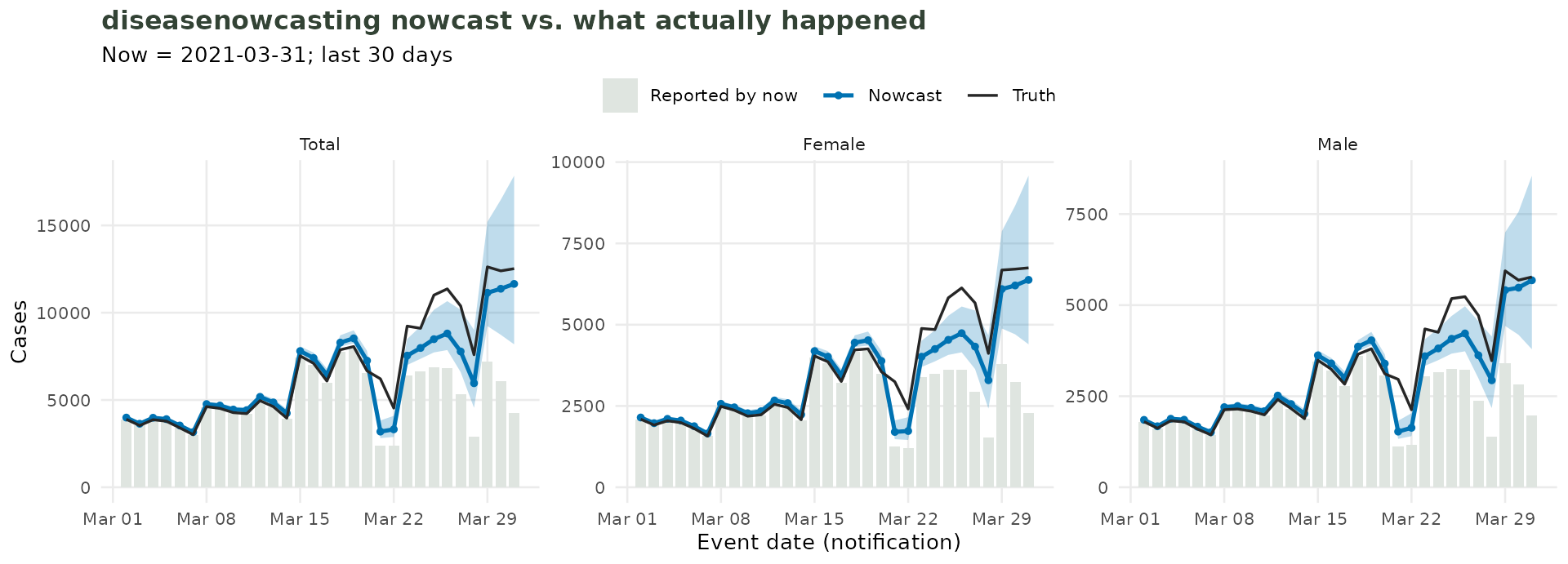 nowcast against the counts reported by now and the counts those dates eventually reached.

Nowcast both stratified and total using the diseasenowcasting package

baselinenowcast

Install with:

install.packages("baselinenowcast")

baselinenowcast is a simple, fast baseline. It works from a reporting triangle, a matrix with one row per event (reference) date and one column per reporting delay. The lower-right corner of the matrix corresponds to the not-yet-observed part the nowcast will fill in.

Simple nowcast

For unstratified data, tbl_now_to_baselinenowcast() builds that triangle directly from the count-incidence data:

library(baselinenowcast)

# Cap the delay axis: a single 185-day straggler gives the
# triangle 186 columns, almost all of them empty.
covid_triangle <- covid_now |>
  tbl_now_to_baselinenowcast(max_delay = 30, verbose = FALSE)

# rows = notification dates, columns = delay in days
covid_triangle[1:5, 1:6]
#>            0 1 2 3 4 5
#> 2020-03-02 0 0 0 0 1 0
#> 2020-03-03 0 0 0 0 0 0
#> 2020-03-06 0 0 0 1 0 0
#> 2020-03-07 0 0 1 0 0 0
#> 2020-03-08 0 0 0 2 0 0

Why cap the delays? The reporting triangle keeps every one of the 393 event dates. Because the maximum delay in our data is 185 days it would mean a matrix of 393 \times 185 = 72,705 entries. This makes the fit extremely slow.

From here you can follow baselinenowcast’s own workflow. For example calling baselinenowcast() to estimate the delay from the triangle, apply it, and draw nowcast samples:

# One-call workflow: estimate the delay, apply it, and draw nowcast samples.
nowcast_samples <- baselinenowcast(
  covid_triangle,
  output_type = "samples",
  draws       = 1000
)

With strata and effects.

baselinenowcast can also take a long tidy data.frame and nowcass every stratum in one call, via its strata_cols argument. Use format = "auto" (the default) or format = "long" on tbl_now_to_baselinenowcast() to get that shape from a stratified tbl_now:

# Long tidy data frame with the strata columns present; `format = "auto"`
# is what `tbl_now_to_baselinenowcast()` returns when the object has strata.
by_stratum <- tbl_now_to_baselinenowcast(
  covid_seasonal,
  max_delay = 30,
  verbose   = FALSE
)

head(by_stratum)
#>   reference_date report_date count    sex .event_day_of_week .event_season_365_cos .event_season_365_sin
#> 1     2020-03-02  2020-03-06     1 Female             Monday             1.0000000            0.00000000
#> 2     2020-03-03  2020-03-14     1 Female            Tuesday             0.9998518            0.01721336
#> 3     2020-03-06  2020-03-09     1   Male             Friday             0.9976303            0.06880243
#> 4     2020-03-07  2020-03-09     1 Female           Saturday             0.9962982            0.08596480
#> 5     2020-03-08  2020-03-11     2 Female             Sunday             0.9946708            0.10310170
#> 6     2020-03-09  2020-03-11     1 Female             Monday             0.9927487            0.12020804

Hand it to baselinenowcast(strata_cols = ...) for one fit per stratum, or opt into strata_sharing = "delay" / "uncertainty" to share the delay PMF or the uncertainty parameters across strata:

# One `baselinenowcast_df` covering every stratum.
nowcasts_by_stratum <- baselinenowcast(
  by_stratum,
  strata_cols = get_strata(covid_seasonal),
  output_type = "samples", draws = 1000
)

In both stratified and unstratified cases the predictions can be recovered with tidy:

tidy(nowcast_samples)

#> # A tibble: 5 × 7
#>   event_date stratum estimate conf.low conf.high level engine         
#>   <date>     <chr>      <dbl>    <dbl>     <dbl> <dbl> <chr>          
#> 1 2021-03-27 all        8439     5833.    15105.  0.95 baselinenowcast
#> 2 2021-03-28 all        4854     3315.     8645.  0.95 baselinenowcast
#> 3 2021-03-29 all       12912     8586.    23755.  0.95 baselinenowcast
#> 4 2021-03-30 all       13386     8821.    22869.  0.95 baselinenowcast
#> 5 2021-03-31 all       15678.    9488.    24488.  0.95 baselinenowcast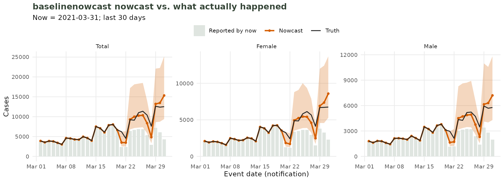

Three panels (Total, Female, Male) comparing the baselinenowcast nowcast against the counts reported by now and the counts those dates eventually reached.

Nowcast both stratified and total using the baselinenowcast package

epinowcast

Install with:

install.packages("epinowcast", repos = c("https://epinowcast.r-universe.dev", getOption("repos")))

# Also requires installation of STAN:
install.packages("cmdstanr", repos = c('https://stan-dev.r-universe.dev', getOption("repos")))

epinowcast fits a flexible Bayesian model with separate modules for the reporting delay and the reference (epidemic) process. It expects a preprocessed object built by enw_preprocess_data().

tbl_now_to_epinowcast() handles the preprocessing, returning an object you can pass straight to epinowcast::epinowcast():

Simple nowcast

epinowcast becomes very slow with the 2.3M cases reporting triangle. So we need to filter earlier, on the observations keeping only the most recent 90 days before applying tbl_now_to_epinowcast().

library(epinowcast)

# Trim, then convert. 90 days otherwise the model is too slow
covid_enw_recent <- covid_now |>
  filter(notification_date >= as.Date("2021-04-01") - 90) |>
  tbl_now_to_epinowcast(max_delay = 30, verbose = FALSE, quiet = TRUE)

covid_enw_recent
#> ── Preprocessed nowcast data ─────────────────────────────────────────────────────────────────────────────────────────────────────────────────────────────────── 
#> Groups: 1 | Timestep: day | Max delay: 30 
#> Observations: 90 timepoints x 90 snapshots 
#> Max date: 2021-03-31 
#> 
#> Datasets (access with `enw_get_data(x, "<name>")`): 
#>   obs                :   2,265 x 7 
#>   new_confirm        :   2,265 x 9 
#>   latest             :      90 x 8 
#>   missing_reference  :       0 x 4 
#>   reporting_triangle :      90 x 32 
#>   metareference      :      90 x 7 
#>   metareport         :     119 x 10 
#>   metadelay          :      30 x 5

This can then be passed to epinowcast():

# A minimal epinowcast fit from the preprocessed object
enw_fit <- epinowcast(
  covid_enw_recent,
  fit = enw_fit_opts(
    pp = TRUE, chains = 1, iter_sampling = 250, iter_warmup = 250,
    seed = 20260824
  )
)

Again, the max_delay is a modelling choice, not a detail: left unset, the converter infers it from the longest delay present, and the nowcast then carries one reference date per delay becoming extremely slow.

With strata and effects.

Handing tbl_now_to_epinowcast() the enriched object does two things automatically: the sex stratum becomes epinowcast’s grouping (by), so the model fits a delay per sex, and the temporal-effect columns land in the metareference / metareport tables so that they can be used in a module formula.

# Same trim, from the enriched object.
enw_seasonal <- covid_seasonal |>
  filter(notification_date >= as.Date("2021-04-01") - 90) |>
  tbl_now_to_epinowcast(max_delay = 30, verbose = FALSE, quiet = TRUE)

# The temporal columns carry the same names as  in `covid_seasonal` after 
# `compute_temporal_effects()`. It can be used in any parametric model
enw_seasonal_fit <- epinowcast(
  enw_seasonal,
  reference = enw_reference(
    parametric   = ~ 1 + .event_day_of_week, 
    distribution = "lognormal",
    data         = enw_seasonal
  ),
  fit = enw_fit_opts(
    pp = TRUE, chains = 1, iter_sampling = 250, iter_warmup = 250,
    seed = 20260824
  )
)

These fits are deliberately small. Two chains, 250 warmup and 250 sampling iterations on a short window, because this page is a tutorial and not a final nowcast.

In both stratified and unstratified cases the predictions can be recovered with tidy:

tidy(enw_fit)

#> # A tibble: 5 × 7
#>   event_date stratum estimate conf.low conf.high level engine    
#>   <date>     <chr>      <dbl>    <dbl>     <dbl> <dbl> <chr>     
#> 1 2021-03-27 all        8350.    6269.    16325.   0.9 epinowcast
#> 2 2021-03-28 all        8322     4173.    20692.   0.9 epinowcast
#> 3 2021-03-29 all       16225     9415.    39159.   0.9 epinowcast
#> 4 2021-03-30 all       21883    10270.    59333.   0.9 epinowcast
#> 5 2021-03-31 all       25545     9765     75139.   0.9 epinowcast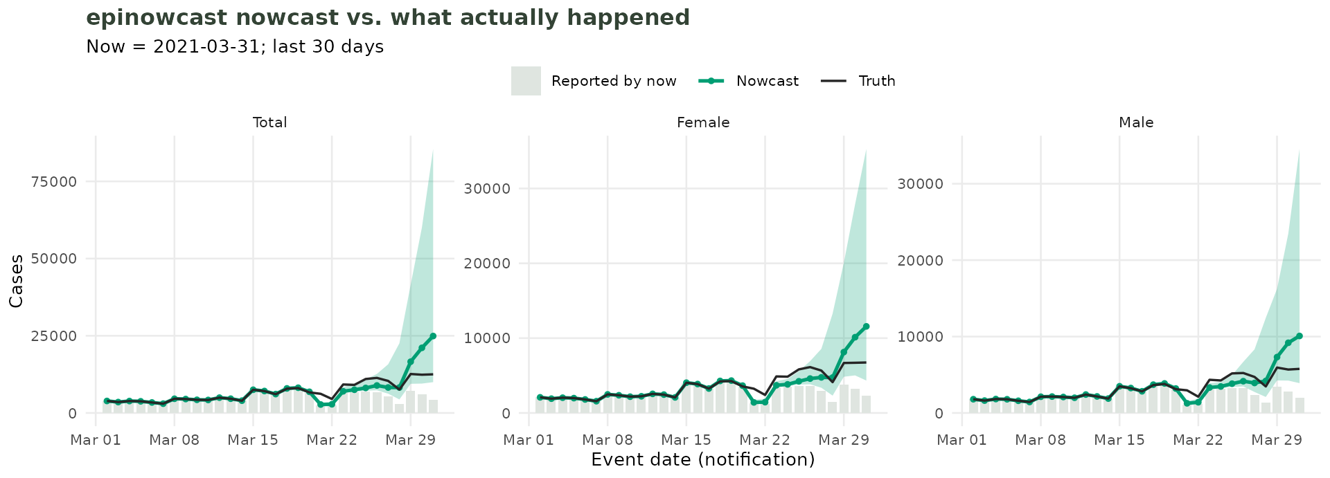

Three panels (Total, Female, Male) comparing the epinowcast nowcast against the counts reported by now and the counts those dates eventually reached.

Nowcast both stratified and total using the epinowcast package

NobBS

Install with:

install.packages("NobBS")

NobBS works from a linelist with an onset-date column and a report-date column, and it counts rows. Each row is one case. Our data are counts, so they have to be expanded first. tbl_now_to_nobbs() does that and names the columns what NobBS() expects:

Simple nowcast

# Trim, then convert. 90 days otherwise the model is too slow
covid_linelist <- covid_now |>
  filter(notification_date >= as.Date("2021-04-01") - 90) |>
  tbl_now_to_nobbs(verbose = FALSE)

nrow(covid_linelist)   # one row per case
#> [1] 651051

We can then nowcast with the built data frame:

library(NobBS)

nobbs_fit <- NobBS(
  data          = covid_linelist,
  now           = get_now(covid_now),
  units         = "1 day",
  onset_date    = "onset_date",
  report_date   = "report_date",
  max_D         = 15,   # delays beyond 15 days are negligible here
  moving_window = 30 
)

The predictions come out with tidy(), in the same shape as every other engine here:

tidy(nobbs_fit)

#> # A tibble: 5 × 7
#>   event_date stratum estimate conf.low conf.high level engine
#>   <date>     <chr>      <dbl>    <dbl>     <dbl> <dbl> <chr> 
#> 1 2021-03-27 all         9248    9070       9420    NA NobBS 
#> 2 2021-03-28 all         5332    5203.      5471    NA NobBS 
#> 3 2021-03-29 all        14458   14199      14727    NA NobBS 
#> 4 2021-03-30 all        14780   14478      15081    NA NobBS 
#> 5 2021-03-31 all        16610   16165      17077    NA NobBS

Notice that even the arguments come from the tbl_now: get_now(), get_event_date() and get_report_date() tell NobBS what tbl.now already figured out.

With strata and effects.

NobBS.strat() fits one nowcast per stratum, and its strata argument names one column. tbl_now_to_nobbs() therefore adds a strata column holding every declared stratum pasted together under the name strata. Use "strata" as the name for NobBS.strat:

covid_linelist_sex <- covid_seasonal |>
  filter(notification_date >= as.Date("2021-04-01") - 60) |>
  tbl_now_to_nobbs(verbose = FALSE) 

stratified_nobbs <- NobBS.strat(covid_linelist_sex,
                                strata        = "strata",
                                now           = get_now(covid_seasonal),
                                units         = "1 day",
                                onset_date    = "onset_date",
                                report_date   = "report_date",
                                max_D         = 15,
                                moving_window = 30
                                )

These fits are deliberately small. A moving window of 30 and a maximum delay of 15 is probably too short for this data. This is done for speed as this page is a tutorial and not a final nowcast.

In both stratified and unstratified cases the predictions can be recovered with tidy:

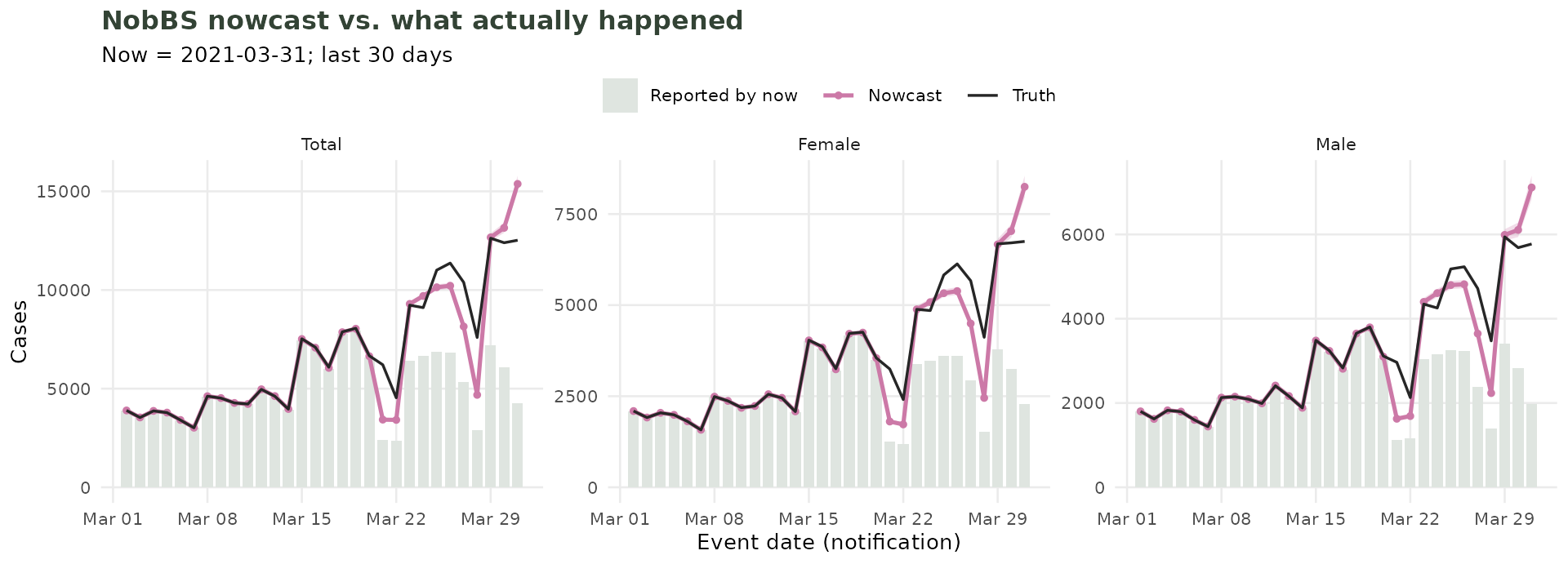
Three panels (Total, Female, Male) comparing the NobBS nowcast against the counts reported by now and the counts those dates eventually reached.

Nowcast both stratified and total using the NobBS package

surveillance

Install with:

install.packages("surveillance")

surveillance is the long-standing R package for outbreak detection and nowcasting, and implements the Höhle & an der Heiden (2014) approach. surveillance::nowcast() works from an individual-level line list with one column for the event date and one for the report date, named by its dEventCol / dReportCol arguments.

tbl_now_to_surveillance() builds that data frame and renames the two dates to surveillance’s own defaults:

Simple nowcast

library(surveillance)

# Trim, then convert. 90 days otherwise the model is too slow
covid_sur_now <- covid_now |>
  filter(notification_date >= as.Date("2021-04-01") - 60)

covid_sur <- tbl_now_to_surveillance(covid_sur_now, verbose = FALSE)

head(covid_sur)
#>    dHospital    dReport
#> 1 2021-01-31 2021-01-31
#> 2 2021-01-31 2021-01-31
#> 3 2021-01-31 2021-01-31
#> 4 2021-01-31 2021-01-31
#> 5 2021-01-31 2021-01-31
#> 6 2021-01-31 2021-01-31

surveillance::nowcast() requires you to pass two date grids. Use get_surveillance_when() to get the dates you want estimated, and get_surveillance_range() for the whole axis the model is laid on. The nowcast itself needs a now, the dates you want estimated (when), and a maximum delay D. All of it can come from the tbl_now:

#Note that in the call we use our get_now(), get_surveillance_when()
#and get_surveillance_range() functions:
sur_fit <- nowcast(
  now          = get_now(covid_sur_now),
  when         = get_surveillance_when(covid_sur_now, length = 30),
  data         = covid_sur,
  dEventCol    = "dHospital",
  dReportCol   = "dReport",
  aggregate.by = "1 day",
  D            = 15,
  method       = "bayes.notrunc.bnb",
  control      = list(dRange = get_surveillance_range(covid_sur_now), 
                      N.tInf.max = 100000, nSamples = 1000)
)

The predictions come out with tidy(), in the same shape as every other engine here:

tidy(sur_fit)

#> # A tibble: 5 × 7
#>   event_date stratum estimate conf.low conf.high level engine      
#>   <date>     <chr>      <dbl>    <dbl>     <dbl> <dbl> <chr>       
#> 1 2021-03-27 all         7355     7251      7462  0.95 surveillance
#> 2 2021-03-28 all         4197     4113      4284  0.95 surveillance
#> 3 2021-03-29 all        11283    11125     11445  0.95 surveillance
#> 4 2021-03-30 all        11540    11337     11746  0.95 surveillance
#> 5 2021-03-31 all        13236    12905     13575  0.95 surveillance

With strata and effects.

surveillance::nowcast() has no strata argument as it only models one series, so a stratified analysis means one fit per stratum. Ask the converter for format = "linelist_list" and it does the splitting: one line list per stratum, in a plain list you can use lapply() over.

# Trim first, as it can't handle the 2.3M cases of the whole window.
covid_sur_seasonal <- covid_seasonal |>
  filter(notification_date >= as.Date("2021-04-01") - 90)

covid_sur_eff <- tbl_now_to_surveillance(
  covid_sur_seasonal,
  format  = "linelist_list",
  verbose = FALSE
)

covid_sur_eff
#> ── 2 surveillance line lists from a <tbl_now> ──────────────────────────────────────────────────────────────────────────────────────────────────────────────────
#> • One per stratum ("sex"): "Female" and "Male"
#> • Date columns: "dHospital" (event), "dReport" (report)
#> • Rows each: 348346 and 302705
#> • Now: "2021-03-31"
#> ℹ `lapply()` over this, passing `control$dRange = get_surveillance_range(x)` from the WHOLE object so every stratum shares one time axis.

With no strata declared this is still a list, of length one named "all", so the lapply() below does not have to know which case it is in. The default format = "linelist" gives the same information as one frame with a pasted strata column, if you would rather split it yourself.

sur_by_stratum <- covid_sur_eff |>
  lapply(\(df) nowcast(
    now          = get_now(covid_sur_seasonal),
    when         = get_surveillance_when(covid_sur_seasonal, length = 30),
    data         = df,
    dEventCol    = "dHospital",
    dReportCol   = "dReport",
    aggregate.by = "1 day",
    D            = 15,
    method       = "bayes.notrunc.bnb",
    control      = list(
      dRange     = get_surveillance_range(covid_sur_seasonal),
      N.tInf.max = 100000,
      nSamples   = 1000
    )
  ))

tidy() recognises the list and labels each block with its own stratum, so sur_by_stratum tidies into one table exactly like the natively stratified engines.

In both stratified and unstratified cases the predictions can be recovered with tidy:

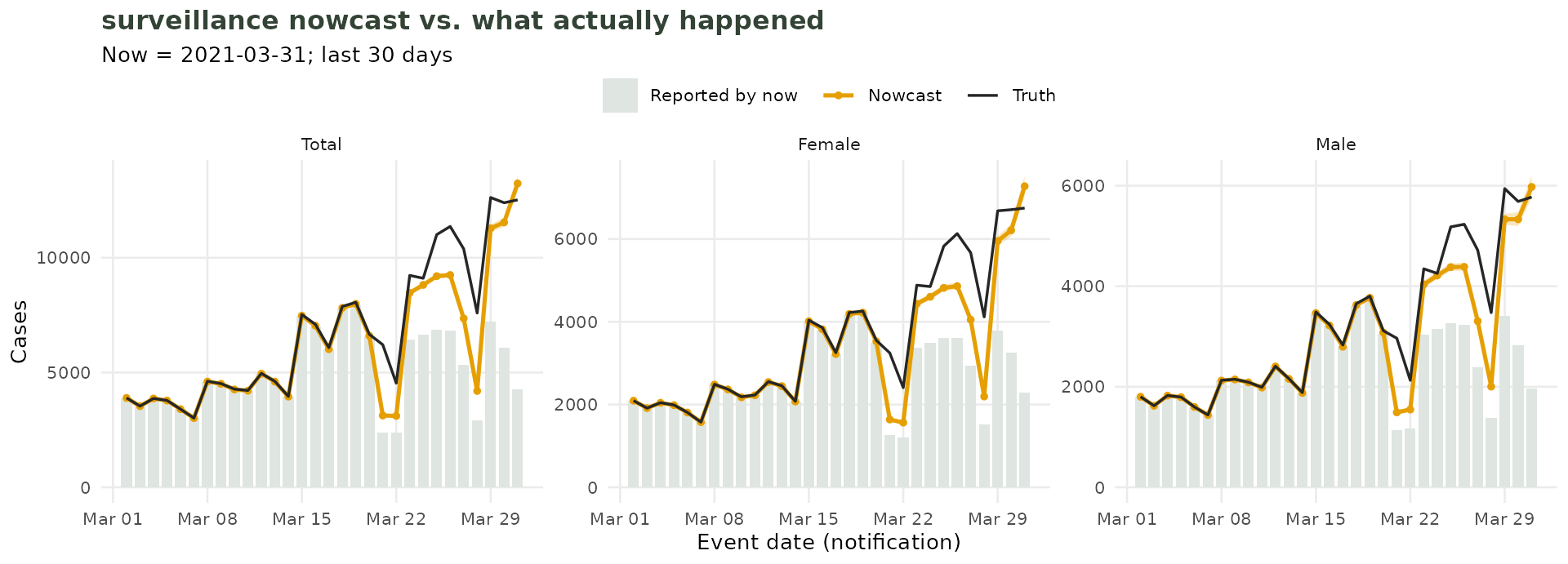
Three panels (Total, Female, Male) comparing the surveillance nowcast against the counts reported by now and the counts those dates eventually reached.

Nowcast both stratified and total using the surveillance package

EpiNow2

Install with:

install.packages("EpiNow2")

EpiNow2 is not a single nowcasting framework but a more general tool that allows you to estimate different distributions related to your epidemic process. The tbl_now_to_EpiNow2() function therefore takes a target argument, named for the function the result is passed to, so whatever it gives you can be handed over unchanged.

`target`	you get	for
`"estimate_infections"` (default)	`date` / `confirm`	`estimate_infections()`, `epinow()`
`"regional_epinow"`	the same plus `region`	`regional_epinow()`
`"estimate_truncation"`	a list of snapshots	`estimate_truncation()`
`"estimate_dist"`	interval-censored date columns	`estimate_dist()`

EpiNow2 models a daily process and has no timestep. To pass weekly data we utilize the accumulate column. Units coarser than a week are refused rather than approximated.

Simple nowcast

estimate_infections() wants the series as known at the now — one row per day, with the filler days marked:

covid_en2 <- covid_now |>
  filter(notification_date >= as.Date("2021-04-01") - 60) |>
  tbl_now_to_EpiNow2(verbose = FALSE, quiet = TRUE)

head(covid_en2)
#>         date confirm
#> 1 2021-01-31    3854
#> 2 2021-02-01    6643
#> 3 2021-02-02    5358
#> 4 2021-02-03    5071
#> 5 2021-02-04    4742
#> 6 2021-02-05    4800

EpiNow2 needs two things fitted before it can nowcast:

delays The infection-to-onset delay which we take from EpiNow2’s shipped example.
truncation is the nowcast itself. That is what the report dimension of a tbl_now measures.

This is a two-step fit.

library(EpiNow2)

# STEP 1 --- fit the truncation from the report dimension.
covid_snaps <- covid_now |>
  filter(notification_date >= as.Date("2021-04-01") - 90) |>
  tbl_now_to_EpiNow2(
    target = "estimate_truncation", snapshots = 5, verbose = FALSE, quiet = TRUE
  )

truncation_fit <- estimate_truncation(
  covid_snaps,
  stan = stan_opts(samples = 250, warmup = 250, chains = 1, seed = 20260824)
)

# `$dist` is defunct; the accessor is `get_parameters()`.
fitted_truncation <- get_parameters(truncation_fit)[["truncation"]]

# STEP 2 --- nowcast with it.
epinow2_fit <- estimate_infections(
  covid_en2,
  generation_time = gt_opts(example_generation_time),
  delays          = delay_opts(example_incubation_period),
  truncation      = trunc_opts(fitted_truncation),
  rt              = rt_opts(prior = LogNormal(mean = 2, sd = 0.1), rw = 7),
  gp              = NULL,
  stan            = stan_opts(samples = 250, warmup = 250, chains = 1, 
                              seed = 20260824)
)

The predictions come out with tidy(), in the same shape as every other engine here:

tidy(epinow2_fit)

#> # A tibble: 5 × 7
#>   event_date stratum estimate conf.low conf.high level engine 
#>   <date>     <chr>      <dbl>    <dbl>     <dbl> <dbl> <chr>  
#> 1 2021-04-03 all        8424     4035.    20402    0.9 EpiNow2
#> 2 2021-04-04 all        6785     2670.    16625.   0.9 EpiNow2
#> 3 2021-04-05 all       10925     5184.    36040.   0.9 EpiNow2
#> 4 2021-04-06 all       12094.    4036.    40879.   0.9 EpiNow2
#> 5 2021-04-07 all       10040     3957.    45165.   0.9 EpiNow2

With strata and effects.

regional_epinow() takes a single region column, so the object’s strata are folded into one label:

covid_regional <- covid_seasonal |>
  filter(notification_date >= as.Date("2021-04-01") - 90) |>
  tbl_now_to_EpiNow2(target = "regional_epinow", verbose = FALSE, quiet = TRUE)

head(covid_regional)
#>         date confirm region
#> 1 2021-01-01    2653 Female
#> 2 2021-01-01    2379   Male
#> 3 2021-01-02    6129 Female
#> 4 2021-01-02    5305   Male
#> 5 2021-01-03    5482 Female
#> 6 2021-01-03    4906   Male

regional_fit <- regional_epinow(
  covid_regional,
  generation_time = gt_opts(example_generation_time),
  delays          = delay_opts(example_incubation_period),
  truncation      = trunc_opts(fitted_truncation),
  rt              = rt_opts(prior = LogNormal(mean = 2, sd = 0.1), rw = 7),
  gp              = NULL,
  stan            = stan_opts(samples = 250, warmup = 250, chains = 1,
                              seed = 20260824)
)

These fits are deliberately small. Two chains, 250 warmup and 250 sampling iterations on a short window, because this page is a tutorial and not a final nowcast.

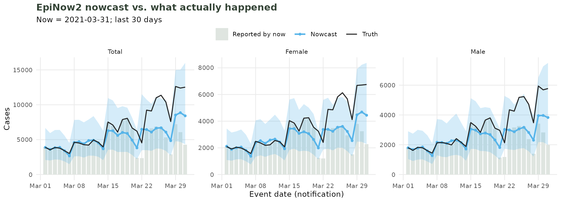
Three panels (Total, Female, Male) comparing the EpiNow2 nowcast against the counts reported by now and the counts those dates eventually reached.

Nowcast both stratified and total using the EpiNow2 package

epidist

Install with:

install.packages("epidist", repos = c('https://epinowcast.r-universe.dev', getOption("repos")))

Sometimes the quantity you actually want is the delay distribution itself. epidist estimates exactly that, treating each case as an interval-censored onset/report pair.

tbl_now_to_epidist() converts the tbl_now into the censored form epidist expects. Our data are daily counts, so the converter produces epidist_aggregate_data with one row per distinct (delay, observation time) combination, and n as that row’s weight. sex is still undeclared on covid_now, and epidist never sees it, so the two rows it splits each cell into are pooled back together here – declaring it (as covid_seasonal does just below) is how you ask for it to reach the model instead.

Simple delay fit

library(epidist)

# Fit the delay distribution (see the epidist documentation for model choices)
delay_model <- covid_now |>
  filter(notification_date >= as.Date("2021-04-01") - 90) |>
  tbl_now_to_epidist(verbose = FALSE) |>
  as_epidist_marginal_model() |>
  epidist(chains = 1, iter = 250, warmup = 250, backend = "cmdstanr")

The fitted delay distribution can then feed back into a nowcast.

With strata and effects.

epidist has no separate grouping argument, so the strata (sex) and the temporal-effect columns become extra columns that can be used within the model’s formula. For example:

# A sex-varying mean delay.
delay_by_sex <- covid_seasonal |>
  filter(notification_date >= as.Date("2021-04-01") - 90) |>
  tbl_now_to_epidist(verbose = FALSE) |>
  as_epidist_marginal_model() |>
  epidist(formula = mu ~ 1 + sex + .event_season_365_sin + .event_season_365_cos,
          chains = 1, iter = 250, warmup = 250, backend = "cmdstanr")

These fits are deliberately small. Two chains, 250 warmup and 250 sampling iterations on a short window, because this page is a tutorial and not a final nowcast.

tidy() works here too, but it returns a slightly different table because epidist estimates a different thing. In this case you get one row per parameter of the fitted delay distribution:

tidy(delay_model)

The `tidy()` function

The converters normalize what goes into each package. tidy() normalizes what comes out. Every engine above returns something different: a matrix of draws, an stsNC object, a Stan fit, an INLA summary, a bare list. The tidy() turns any of them into the same table:

tidy(nowcast_samples)

#> # A tibble: 5 × 7
#>   event_date stratum estimate conf.low conf.high level engine         
#>   <date>     <chr>      <dbl>    <dbl>     <dbl> <dbl> <chr>          
#> 1 2021-03-27 all        8439     5833.    15105.  0.95 baselinenowcast
#> 2 2021-03-28 all        4854     3315.     8645.  0.95 baselinenowcast
#> 3 2021-03-29 all       12912     8586.    23755.  0.95 baselinenowcast
#> 4 2021-03-30 all       13386     8821.    22869.  0.95 baselinenowcast
#> 5 2021-03-31 all       15678.    9488.    24488.  0.95 baselinenowcast

The columns are the same regardless of the package that produced the fit:

column	meaning
`event_date`	event/reference date, on the engine’s own grid
`stratum`	`"all"` when the fit is unstratified
`estimate`	point nowcast (posterior median where available)
`conf.low`, `conf.high`	interval bounds, using ’s names
`level`	the width that interval actually has
`engine`	which package produced it
`qXX`	(optional) quantile columns of the prediction

Pass probs for columns with other quantiles:

tidy(nowcast_samples, probs = c(0.05, 0.5, 0.95))

#> # A tibble: 5 × 10
#>   event_date stratum estimate conf.low conf.high level engine              q5    q50    q95
#>   <date>     <chr>      <dbl>    <dbl>     <dbl> <dbl> <chr>            <dbl>  <dbl>  <dbl>
#> 1 2021-03-27 all        8439     5833.    15105.  0.95 baselinenowcast  6026.  8439  13567.
#> 2 2021-03-28 all        4854     3315.     8645.  0.95 baselinenowcast  3450.  4854   7898.
#> 3 2021-03-29 all       12912     8586.    23755.  0.95 baselinenowcast  8935. 12912  21308.
#> 4 2021-03-30 all       13386     8821.    22869.  0.95 baselinenowcast  9305. 13386  21197.
#> 5 2021-03-31 all       15678.    9488.    24488.  0.95 baselinenowcast 10327. 15678. 22740.

Only engines that keep draws can answer an arbitrary probs. That is diseasenowcasting, baselinenowcast and epinowcast. NobBS and surveillance report a fixed set of summaries, so asking them for a quantile they never computed is an error . To be able to do so you need to specify at fit time the quantiles you want. For example with NobBS you can use the specs to set quantiles:

nobbs_quantiles <- NobBS(
  data          = covid_linelist,
  now           = get_now(covid_now),
  units         = "1 day",
  onset_date    = "onset_date",
  report_date   = "report_date",
  max_D         = 10,
  moving_window = 104,
  specs         = list(quantiles = c(0.1, 0.5, 0.9))   # <- ask here
)

so that they can be called with tidy:

tidy(nobbs_quantiles, probs = c(0.1, 0.5, 0.9))

#> # A tibble: 5 × 7
#>   event_date stratum estimate conf.low conf.high level engine
#>   <date>     <chr>      <dbl>    <dbl>     <dbl> <dbl> <chr> 
#> 1 2021-03-27 all            0        0         0    NA NobBS 
#> 2 2021-03-28 all            0        0         0    NA NobBS 
#> 3 2021-03-29 all            0        0         0    NA NobBS 
#> 4 2021-03-30 all            0        0         1    NA NobBS 
#> 5 2021-03-31 all            0        0         1    NA NobBS

Summary

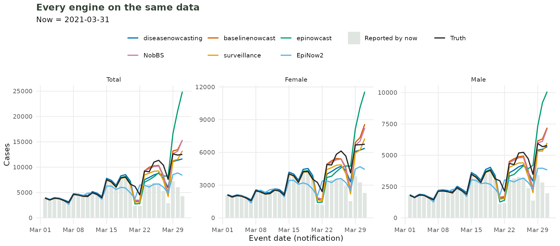
Three panels (Total, Female, Male). Grey bars show the counts reported by now, a dark line the counts those dates eventually reached, and one coloured line per package its nowcast.

We described the data once as a tbl_now, and then a single converter call (or, for diseasenowcasting, no call at all) handed it to each package in the shape it needed:

covid_now <- tbl_now(covid_colombia,
                     event_date  = notification_date,
                     report_date = diagnosis_date,
                     case_count  = n,
                     data_type   = "count-incidence")

covid_now                              # diseasenowcasting
tbl_now_to_baselinenowcast(covid_now)  # baselinenowcast
tbl_now_to_epinowcast(covid_now)       # epinowcast
tbl_now_to_epidist(covid_now)          # epidist
tbl_now_to_surveillance(covid_now)     # surveillance
tbl_now_to_nobbs(covid_now)            # NobBS
tbl_now_to_EpiNow2(covid_now)          # EpiNow2
as.data.frame(covid_now)               # others

Attaching strata and temporal effects once (covid_seasonal) uses the same converters: each package receives them in whatever way it can use.

If you have any questions or comments regarding the contents of this article please open an issue on Github.

Learning more

A tutorial on real life surveillance data. Takes you from cleaning to diagnosing errors in the data to nowcasting: https://rodrigozepeda.github.io/tbl.now/articles/example.html
The second part of the tutorial with a revision process: the optional third date, where a reported case is later confirmed, retracted or left pending: https://rodrigozepeda.github.io/tbl.now/articles/example_revisions.html
The Get started vignette: the whole workflow, from a raw line list to a scored nowcast, in five minutes: https://rodrigozepeda.github.io/tbl.now/articles/tbl.now.html.
More on the tbl_now object: every attribute, the three data types, the revision process, temporal effects and the dplyr methods: https://rodrigozepeda.github.io/tbl.now/articles/more-on-tbl-now.html
More thoughts on diagnosing your dataset with tbl.now https://rodrigozepeda.github.io/tbl.now/articles/diagnosing-a-tbl-now.html
Detecting reporting batches with tbl.now https://rodrigozepeda.github.io/tbl.now/articles/batches.html
How to use different nowcasting engines from tbl.now: here you can learn how it connects to the other nowcasting packages. https://rodrigozepeda.github.io/tbl.now/articles/nowcasting-models.html
How to nowcast with multiple engines, backtest and ensemble nowcasts. https://rodrigozepeda.github.io/tbl.now/articles/ensemble-nowcasting.html
Adding your own custom nowcasting model https://rodrigozepeda.github.io/tbl.now/articles/custom-nowcast-models.html
Package reference: https://rodrigozepeda.github.io/tbl.now/reference/

Why this vignette?

The data

A more complex object: strata and temporal effects

diseasenowcasting

Simple nowcast

With strata and effects.

baselinenowcast

Simple nowcast

With strata and effects.

epinowcast

Simple nowcast

With strata and effects.

NobBS

Simple nowcast

With strata and effects.

surveillance

Simple nowcast

With strata and effects.

EpiNow2

Simple nowcast

With strata and effects.

epidist

Simple delay fit

With strata and effects.

The tidy() function

Summary

Learning more

The `tidy()` function