Batch detection

What this vignette is about

Surveillance systems stall. A laboratory closes over a holiday, a data pipeline breaks for a week, a reporting office falls behind and then catches up. When the system restarts, a backlog of reports arrives all at once. We call that report date a batch.

Batches matter because they look exactly like an epidemic taking off — a sudden jump in reported cases — while being nothing of the sort. A nowcasting model that assumes a stable reporting process will happily interpret a batch as a surge in incidence.

This vignette shows how to find them. Everything here is model-free: no model is fitted and nothing is estimated by a downstream nowcaster. You need only a tbl_now, which makes these tools appropriate for exploratory data analysis before you commit to a model.

The batch-detection functions are experimental: the statistical behaviour and the interface may still change, and each warns you when called. Treat a flagged report date as a potential batch, not a confirmed one.

The theory and its proofs live in the help pages — every function has a “The mathematics” section (see ?batch_screen, ?batch_shape_test, ?simulate_batch). This article is about using them.

library(tbl.now)
library(dplyr)
library(ggplot2)

The one idea you need

A batch moves reports. It does not create them.

Suppose the desk was shut on Monday, Tuesday and Wednesday and reopened on Thursday. Then Thursday reports its own cases plus three days of backlog. But if you draw a box around Monday–Thursday and count everything inside, you get exactly what you would have got with no closure at all. Nothing was invented; things merely arrived on a different day.

A genuine epidemic surge is different: it creates cases, and the box count goes up.

batch_screen() computes exactly these two quantities for every report date:

quantity	meaning	what it detects
`deficit`	reports that went missing in the days before	transport (a batch)
`delta`	the box total minus what we expected	creation (a real surge)

and reads the diagnosis off a 2×2 table:

	`deficit` ≈ 0	`deficit` ≫ 0
`delta` ≈ 0	nothing happened	`"batch"`
`delta` ≫ 0	`"surge"`	`"batch_and_surge"`
`delta` < 0	—	`"hold_or_deletion"` (the stall has not cleared)

Example 1 — Dengue with a planted batch

We start with real dengue data and plant a batch ourselves, so that we know the right answer.

data(denguedat, package = "tbl.now")

dengue_tbl <- denguedat |>
  filter(report_week <= as.Date("1991-06-01")) |>
  tbl_now(
    event_date  = onset_week,
    report_date = report_week,
    data_type   = "linelist",
    verbose     = FALSE
  )

Planting a batch

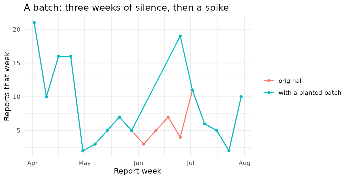
simulate_batch() closes the reporting desk on the dates you name and releases everything on the next open date. It never changes an event date and never moves a report earlier — it is a transport, exactly as the theory defines one.

closed_weeks <- as.Date(c("1990-06-04", "1990-06-11", "1990-06-18"))
release_week <- as.Date("1990-06-25")

dengue_batched <- simulate_batch(dengue_tbl, closed_dates = closed_weeks)

Here is what that did to the report axis. Note the three empty weeks and the spike that pays for them.

Screening for it

screened <- batch_screen(dengue_batched, lookback = 3)
screened
#> # A tibble: 74 × 16
#>    report_date stratum reported baseline window_total window_mean deficit delta
#>  * <date>      <chr>      <dbl>    <dbl>        <dbl>       <dbl>   <dbl> <dbl>
#>  1 1990-01-01  all            3     NA             NA        NA      NA    NA  
#>  2 1990-01-08  all           26     NA             NA        NA      NA    NA  
#>  3 1990-01-15  all           62     NA             NA        NA      NA    NA  
#>  4 1990-01-22  all           41     43.7          132       196.     61.4 -64.1
#>  5 1990-01-29  all           40     31            169       136     -24    33  
#>  6 1990-02-05  all           36     23.2          179        97.8   -68.4  81.2
#>  7 1990-02-12  all           35     24.8          152       108.    -33.9  44.1
#>  8 1990-02-19  all           33     21.4          144        90.9   -41.5  53.1
#>  9 1990-02-26  all           15     22.8          119        99.9   -26.9  19.1
#> 10 1990-03-05  all           21     25.5          104       114       5.5 -10  
#> # ℹ 64 more rows
#> # ℹ 8 more variables: window_scale <dbl>, deficit_scale <dbl>,
#> #   p_creation <dbl>, p_deletion <dbl>, p_transport <dbl>,
#> #   p_transport_bh <dbl>, classification <chr>, batch <lgl>

batch_screen() found the release week and nothing else. Look at what happened around the closure:

screened |>
  filter(report_date >= as.Date("1990-06-04"), report_date <= as.Date("1990-07-02")) |>
  select(report_date, reported, baseline, deficit, delta, classification)
#> # A tibble: 5 × 6
#>   report_date reported baseline deficit delta classification  
#>   <date>         <dbl>    <dbl>   <dbl> <dbl> <chr>           
#> 1 1990-06-04         0     9.67   15.7  -25.3 hold_or_deletion
#> 2 1990-06-11         0     9.88   20.0  -29.9 hold_or_deletion
#> 3 1990-06-18         0    10.0    25    -35.1 hold_or_deletion
#> 4 1990-06-25        19     8.5    24    -13.5 batch           
#> 5 1990-07-02        11     8.09    2.91   0   none

Three things to notice, and they are the whole method:

During the closure the verdict is "hold_or_deletion". delta is strongly negative: reports have gone missing and no spike has yet arrived to pay for them. That is the correct read of a stall in progress.
At the release week, reported is far above baseline and deficit is large — but delta is small. The window total is essentially unchanged. Mass moved; it was not created. Verdict: "batch".
deficit is roughly the number of reports actually withheld. It is not a p-value; it is an estimate of the size of the backlog.

`delta` really is blind to the batch

The central claim of the theory is that delta cannot see a transport confined to its window. This is not an approximation — it is a pathwise identity, and we can check it exactly:

screened_clean <- batch_screen(dengue_tbl, lookback = 3)

delta_clean   <- screened_clean$delta[screened_clean$report_date == release_week]
delta_batched <- screened$delta[screened$report_date == release_week]

c(clean = delta_clean, batched = delta_batched, identical = delta_clean == delta_batched)
#>     clean   batched identical 
#>     -13.5     -13.5       1.0

Identical, to the last digit. Planting a batch changed the reported counts, the baseline, and the deficit — and left delta exactly where it was. That is why delta can be trusted to answer “was anything created here?” even in the presence of a batch.

Looking at who was reported, not just how many

batch_screen() counts reports. batch_shape_test() asks a complementary question: did the reports arriving on this date come from unusually old event dates? A released backlog is old, so its delays should be inflated.

It compares the delays on the candidate date against those of nearby report dates, using a permutation test. Set guard to skip the dates immediately around the candidate — those are the deficit weeks, and including them would contaminate the comparison.

batch_shape_test(dengue_batched, at = release_week, guard = 3, seed = 1)
#> # A tibble: 1 × 7
#>   stratum  n_at n_reference mean_delay_at mean_delay_reference statistic p_value
#>   <chr>   <int>       <int>         <dbl>                <dbl>     <dbl>   <dbl>
#> 1 all        19          45          3.58                 2.33      1.68   0.041

The mean delay at the release week is substantially longer than at its neighbours, and the permutation test rejects. On the original data, the same date is unremarkable:

batch_shape_test(dengue_tbl, at = release_week, guard = 3, seed = 1)
#> # A tibble: 1 × 7
#>   stratum  n_at n_reference mean_delay_at mean_delay_reference statistic p_value
#>   <chr>   <int>       <int>         <dbl>                <dbl>     <dbl>   <dbl>
#> 1 all         4          41             1                 2.02     -1.06   0.879

This test is remarkable for how little it assumes: it needs neither the reporting delay distribution nor the epidemic curve. It only needs the epidemic to be locally log-linear, which any smooth curve is. See the “The mathematics” section of ?batch_shape_test for why.

Example 2 — Count-cumulative data (FluSight)

Some surveillance streams publish a running cumulative total for each week, re-reported over time, which can be revised down as well as up. FluSight hospitalisations are one such stream. Batch detection works there too — the theory is about transport, and transport does not care whether the increments are signed.

data(flusight, package = "tbl.now")

flusight_tbl <- flusight |>
  filter(location_name == "California",
         as_of >= as.Date("2023-10-01"), as_of <= as.Date("2024-06-01"),
         observation >= 0) |>
  tbl_now(
    event_date  = target_end_date,
    report_date = as_of,
    case_count  = observation,
    data_type   = "count-cumulative",
    verbose     = FALSE
  )

get_data_type(flusight_tbl)
#> [1] "count-cumulative"

batch_screen() de-accumulates the cumulative curve into the signed increment each report announced, then proceeds exactly as before. Because the increments are signed, the window total is a difference of counting processes rather than a count, so the exact Poisson reference is replaced by a robust normal approximation. You do not have to ask for this; it is chosen from the data type.

flusight_batched <- simulate_batch(
  flusight_tbl,
  closed_dates = as.Date(c("2024-01-13", "2024-01-20"))
)

flusight_screened <- batch_screen(flusight_batched, lookback = 2)
attr(flusight_screened, "null_model")
#> [1] "robust"

flusight_screened |>
  filter(report_date >= as.Date("2023-12-30"), report_date <= as.Date("2024-02-10")) |>
  select(report_date, reported, baseline, deficit, delta, classification)
#> # A tibble: 7 × 6
#>   report_date reported baseline deficit delta classification  
#>   <date>         <dbl>    <dbl>   <dbl> <dbl> <chr>           
#> 1 2023-12-30      1720    1096.   -698  1322. surge           
#> 2 2024-01-06      1424     439.  -2505. 3490. surge           
#> 3 2024-01-13         0     542.  -1942. 1399. surge           
#> 4 2024-01-20         0     577.   -140. -437. hold_or_deletion
#> 5 2024-01-27      2795     551.   1287   957. batch_and_surge 
#> 6 2024-02-03       542     494.  -1643. 1690. surge           
#> 7 2024-02-10       405     409.  -2395. 2391  surge

The release date is flagged. But notice it is called "batch_and_surge", and the weeks around it are called "surge". That is correct, and worth understanding.

Late January 2024 is the peak of the influenza season: cases really were being created, fast. delta measures creation relative to a line extrapolated from outside the window, and an exponential epidemic rise is not a straight line. So "surge" fires — on the original data too:

flusight_clean <- batch_screen(flusight_tbl, lookback = 2)

peak_week <- as.Date("2024-01-27")
tibble(
  quantity = c("delta", "deficit"),
  clean    = c(flusight_clean$delta[flusight_clean$report_date == peak_week],
               flusight_clean$deficit[flusight_clean$report_date == peak_week]),
  batched  = c(flusight_screened$delta[flusight_screened$report_date == peak_week],
               flusight_screened$deficit[flusight_screened$report_date == peak_week])
)
#> # A tibble: 2 × 3
#>   quantity clean batched
#>   <chr>    <dbl>   <dbl>
#> 1 delta     957.    957.
#> 2 deficit  -802    1287

Read that table carefully, because it is the method in miniature:

delta is identical in the clean and batched data. The epidemic peak is real and delta sees it; the batch is invisible to delta.
deficit swings from negative to strongly positive. The batch is entirely visible to deficit.

So "surge" came from the flu peak and "batch" came from our planted stall. The classifier is telling the truth about both.

The surge verdict is the weaker one. The transport test conditions on the window total, so it does not care what the underlying intensity is or how good the baseline is. The creation test compares against the baseline directly, and is therefore only as good as it. On a steeply curving epidemic curve, "surge" will fire on ordinary growth. If you want to detect genuine surges, fit a model. If you want to detect batches, this screen is the right tool.

Example 3 — Weekends, holidays and other schedules

A reporting system that is always closed at weekends produces every batch symptom, every single week. This is a scheduled transport, and it is not what we are hunting. Left unmodelled it will flood the screen with false positives.

Here is daily data whose weekend reports are pushed to Monday.

set.seed(42)

origin_dates <- seq(as.Date("2021-01-04"), by = "day", length.out = 120)
report_rows  <- vector("list", length(origin_dates))

for (origin_index in seq_along(origin_dates)) {
  origin_date <- origin_dates[origin_index]
  n_cases     <- rpois(1, 30)
  if (n_cases == 0) next

  report_date <- origin_date + rgeom(n_cases, prob = 0.5)
  # The desk is shut at weekends: those reports slide to the following Monday.
  weekday     <- as.POSIXlt(report_date)$wday
  report_date <- report_date + ifelse(weekday == 6, 2, ifelse(weekday == 0, 1, 0))

  report_rows[[origin_index]] <- data.frame(onset = origin_date, report = report_date)
}

scheduled_tbl <- bind_rows(report_rows) |>
  filter(report <= as.Date("2021-05-01")) |>
  tbl_now(event_date = onset, report_date = report,
          data_type = "linelist", verbose = FALSE)

Screen it twice — once naively, once telling batch_screen() that the cycle is seven days long:

naive    <- batch_screen(scheduled_tbl, lookback = 3)
adjusted <- batch_screen(scheduled_tbl, lookback = 3, period = 7)

c(
  "flagged without `period`" = sum(naive$batch,    na.rm = TRUE),
  "flagged with `period = 7`" = sum(adjusted$batch, na.rm = TRUE)
)
#>  flagged without `period` flagged with `period = 7` 
#>                        17                         0

Every Monday is a phantom batch until the schedule is modelled; afterwards, none of them are. batch_screen() estimates the effect of each phase of the cycle by taking medians across cycles, which recovers the schedule as long as irregular batches hit any given phase in fewer than half of its cycles.

Now plant a real, irregular four-day stall on top of the weekly schedule and see whether it can still be found:

irregular_closure <- as.Date(c("2021-03-08", "2021-03-09", "2021-03-10", "2021-03-11"))

scheduled_batched <- simulate_batch(scheduled_tbl, closed_dates = irregular_closure,
                                    verbose = FALSE)

batch_screen(scheduled_batched, lookback = 4, period = 7) |>
  filter(batch) |>
  select(report_date, reported, baseline, deficit, delta, classification)
#> # A tibble: 1 × 6
#>   report_date reported baseline deficit delta classification
#>   <date>         <dbl>    <dbl>   <dbl> <dbl> <chr>         
#> 1 2021-03-12       208     28.0    160.  19.7 batch

The release date (12 March) is recovered. Always pass period when your reporting system has a fixed cycle.

Practical guidance

Choosing lookback. This is the width of the box. It must comfortably cover the longest stall you think plausible: a three-day closure needs lookback >= 3. Too small and the deficit falls outside the window; too large and you lose power, because the box total gets noisier. When in doubt, try a few values — a real batch survives.

Choosing baseline_window. It must satisfy baseline_window >= 2 * lookback + 3, which batch_screen() enforces, so that a batch episode can never outvote the robust baseline it is being measured against. The default is the smallest admissible value.

Reading the output.

batch is the flag you should act on: it applies a Benjamini–Hochberg correction across every (report date, stratum) pair.
classification uses raw p-values, so it is more liberal. It is there to tell you which kind of anomaly, not whether.
Flags often cluster around an episode. One stall may light up its release date and a neighbour; that is expected, not a second batch.

Strata. A batch is a report date that is anomalous for at least one stratum — one laboratory can stall while others do not. batch_screen() returns one row per (report date, stratum) and corrects across all of them.

What this will not do. If a stall has not cleared by the end of your data, you see the lull and never the spike. Within the data you have, that is indistinguishable from cases being deleted — an honest impossibility, not a failure of the method. batch_screen() labels it "hold_or_deletion" rather than guessing.

A batch is not a single strange report. It is tempting to look for one case with a shockingly long delay. But a batch produces many cases with mildly inflated delays — a whole backlog, each a few days late. Finding one huge departure and finding many small ones are different statistical problems: the former wants a maximum, the latter wants to accumulate the small pieces of evidence, which is exactly what the volume/deficit contrast and the rank-sum shape test do. A per-report outlier rule (useful in its own right for spotting a single mis-recorded delay) is the wrong instrument here.

Use each tool for its question:

question	tool
Did this report date release a backlog?	`batch_screen()`
Did this report date draw on unusually old cases?	`batch_shape_test()`
Is this individual report implausibly delayed?	see `test_delay_drift()` and downstream model-based checks

tbl.now team

What this vignette is about

The one idea you need

Example 1 — Dengue with a planted batch

Planting a batch

Screening for it

`delta` really is blind to the batch

Looking at who was reported, not just how many

Example 2 — Count-cumulative data (FluSight)

Example 3 — Weekends, holidays and other schedules

Practical guidance

See also

Batch detection

tbl.now team

What this vignette is about

The one idea you need

Example 1 — Dengue with a planted batch

Planting a batch

Screening for it

delta really is blind to the batch

Looking at who was reported, not just how many

Example 2 — Count-cumulative data (FluSight)

Example 3 — Weekends, holidays and other schedules

Practical guidance

See also

`delta` really is blind to the batch