Nowcasting methods

Intuitive explanation

We consider the problem of reporting the number of cases for a certain disease. Results of disease’s tests are reported with a delay. So for any day we will see only some disease-cases in that day; other disease-cases for the same day will be reported in the upcoming days.

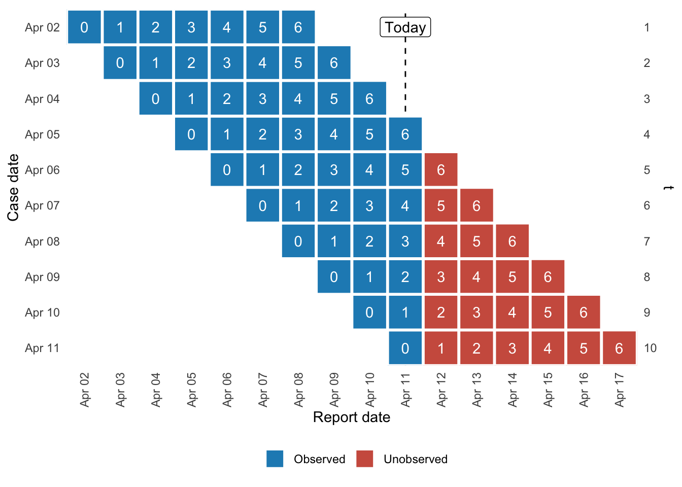
Delay ladder shows that by each day the reports come in the subsequent days thus forming a ladder.

Figure 1 shows this idea where we assume that the maximum delay corresponds to $6$ days. We can see that by today, April 11th, all of the data for April the 2nd has already arrived: the data that arrived with zero delay (report Apr. 2) as well as the data that arrived with a delay of $1$ (report Apr. 3), $2$ (report Apr. 4), $3$ (report Apr. 5), etc until the data that was reported on April 8th with the maximum delay of 6. For other dates not all data has yet arrived. We can see that for April 9th we only see the data with delay 0 up till 3 (corresponding to April 11th). Data with delay larger than 3 will be seen in the future.

The idea of the model is to predict the number of cases that will be seen at time $t$ denoted $n_{t}$ as the sum of the delayed cases. This includes both the cases we’ve already observed $n_{t,d}$ and the cases we haven’t yet observed $\tilde{n}_{t,d}$.

The number of cases at time $t$, $n_t$ can be decomposed into those observed with delays $0$ (no delay), and $1,2,3$, $n_{t,0},n_{t,1},n_{t,2},n_{t,3}$ and those predicted for delays $4,5,6$: $n_{t,4},n_{t,5},n_{t,6}$

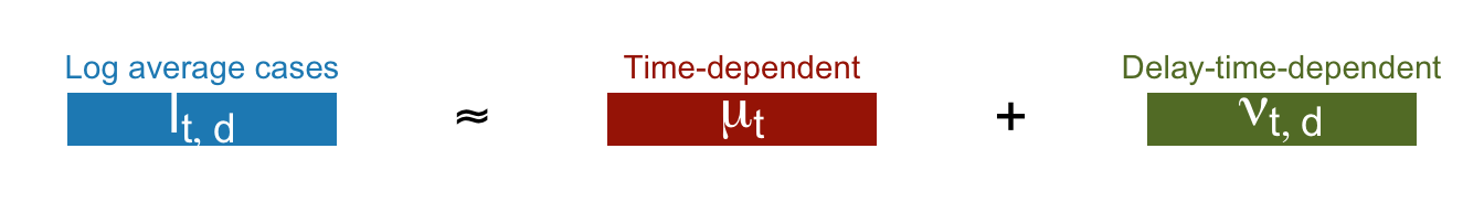
The main objective is then to model $n_{t,d}$, the number of cases at time $t$ that will appear with delay $d$. What we actually model is the log expected value of $n_{t,d}$, denoted $\ell_{t,d}$. The average of this variable is driven by a process composed of two elements: a time-dependent process and a delay-time-dependent process. You can think of the time-dependent process as the process that drives the epidemic curve while the delay-time-dependent process is the process that drives the testing (or changes in the testing).

The log expected number of cases at time $t$ reported with delay $d$, $\ell_{t,d}$ is a function of a time-dependent process $\mu_t$ and a delay-time-dependent process $\nu_{t,d}$.

Each of the processes can be further decomposed into a trend, a season (or multiple seasons), and a cycle:

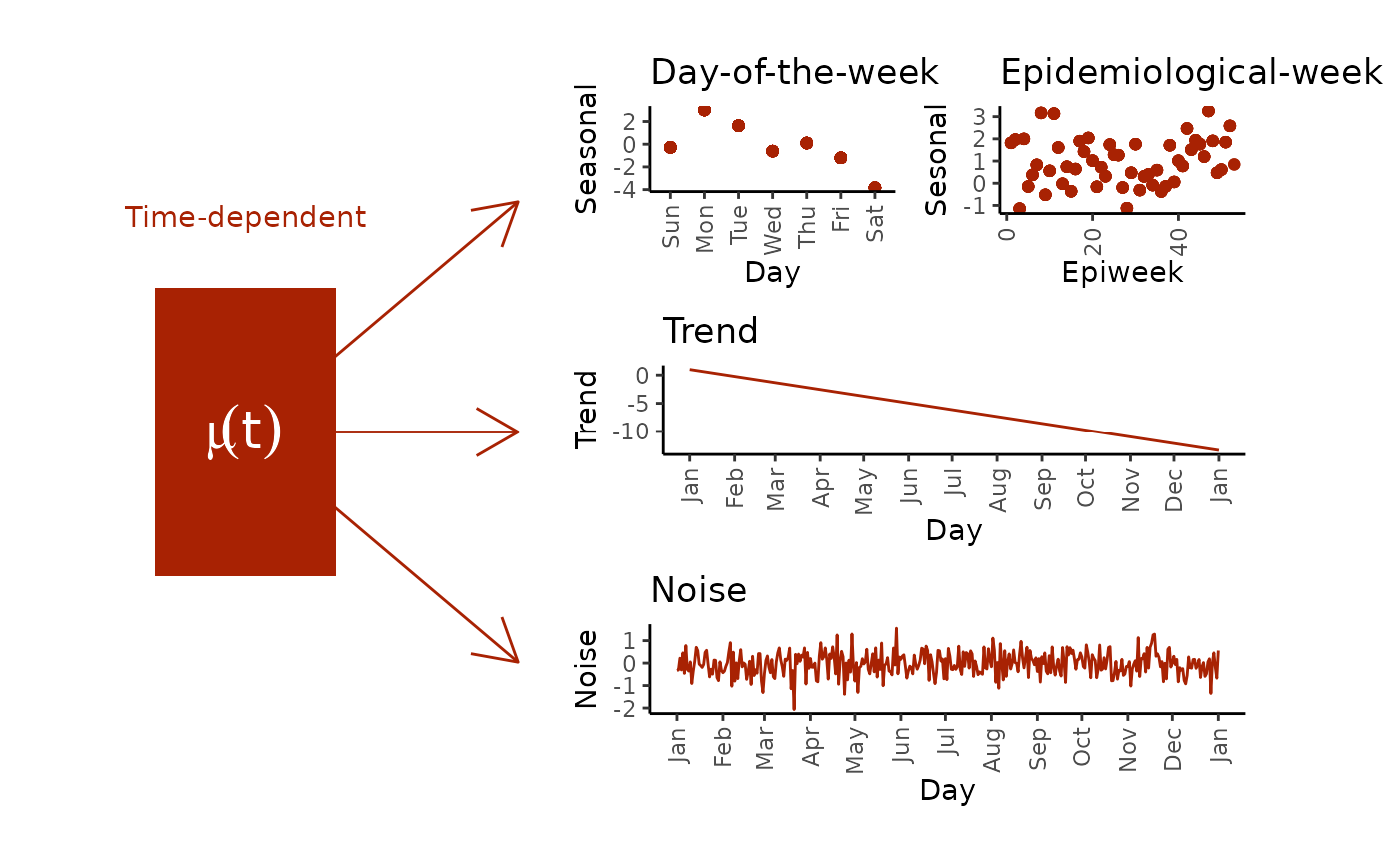
The decomposition of the time-dependent process $\mu_t$. The delay-time-dependent process $\nu_{t,d}$ is decomposed in a similar fashion.

The model thus captures seasonality both for the epidemic curve and for the delay curve as well as their own trends and noise.

Mathematical explanation

Let $n_{t,d}^s$ denote the number of incident cases (individuals) in stratum $s$ (say race/gender) at time $t$ who were reported with a delay $d$. That is, $n_{t,0}$ denotes the the number of individuals diseased at time $t$ that were reported at moment $t$, $n_{t,1}$ the number of individuals diseased at time $t$ that were reported at moment $t + 1$ and in general $n_{t,d}$ the number of individuals diseased at time $t$ that were reported at moment $t + d$.

We assume that the expected value of $n_{t,d}^s$ is given by: $$\mathbb{E}\left[n_{t,d}^s\right] = \lambda_{t,d}^s$$ where $\ell_{t,d}^s = \ln\lambda_{t,d}^s$ follows a linear state-space model with covariates (see Durbin and Koopman (2012)):

$$\begin{equation} \begin{aligned} \ell_{t,d}^s & = L^{\mu} \cdot \mu_{t}^s + L_{d}^{\nu} \cdot \nu_{t,d}^s + B_{d} \cdot X_{t,d}^s + \epsilon_{t,d}^s \\ \mu_{t+1}^s & = A^{\mu} \mu_{t}^s + R^{\mu} \xi_{t}^{s,\mu} \quad & \text{(time-dependent process)}\\ \nu_{t+1,d}^s & = A_{d}^{\nu}\nu_{t,d}^s + R_d^{\nu} \xi_{t,d}^{s,\nu} \quad & \text{(delay-dependent process)}\\ \end{aligned} \end{equation}$$

where $\mu_{t}^s$ represents the time-dependent latent process and $\nu_{t,d}^s$ the delay-dependent latent process. The system is defined for $t = 1,\dots, T$ (time), $d = 0,\dots, D$ (delays) and $s = 1,\dots,S$ (strata). Table 1 describes each of the variables and their dimensions.

Dimensions of variables.

Variable(s)	Dimension
$A^{\mu}$	$(r_{\mu} \times p_{\mu})$
$A_{d}^{\nu}$	$(r_{\nu} \times p_{\nu})$
$R^{\mu}$	$(r_{\mu} \times r_{\mu})$
$R_d^{\nu}$	$(r_{\nu} \times r_{\nu})$
$B_{d}$, $X_{t,d}^s$	$(q \times 1)$
$L^{\mu}$, $\mu_{t+1}^s$	$(r_{\mu} \times 1)$
$L_d^{\nu}$, $\nu_{t+1,d}^s$	$(r_{\nu} \times 1)$
$\epsilon_{d,t}^{s}$	$(1 \times 1)$
$\xi_{d,t}^{s,\mu}$	$(r_{\mu} \times 1)$
$\xi_{d,t}^{s,nu}$	$(r_{\nu} \times 1)$

In this model, $A^{\mu}$,$A_{d}^{\nu}$, $R^{\mu}$,$R_d^{\nu}$,$L^{\mu}$, and $L_d^{\nu}$ are given. Variables $\epsilon_{t,d}^s$, $\xi_{t}^{s,\mu}$, and $\xi_{t,d}^{s,\nu}$ represent random (correlated) noise; $X_{t,d}^s$ is a vector of known covariates, $B_d$ is a vector of unknown parameters. Additionally, $\mu_{0}$ and $\nu_{0,d}$ are also unknown parameters.

The total number of incident cases for stratum $s$ expected to at time $t$ is given by: $$\begin{equation} n_t^s = \sum\limits_{d = 0}^{\infty} n_{t,d}^s = n_{t,D+}^s + \sum\limits_{d = 0}^{D} n_{t,d}^s \approx \sum\limits_{d = 0}^{D} n_{t,d}^s \end{equation}$$ At time $t$, the predicted number of cases with delay $d$ of stratum $s$ is denoted by $\tilde{n}_{t,d}^s$. Finally, the predicted number of cases (nowcasted cases) in stratum $s$ for time $t$ is estimated by: $$\begin{equation} \tilde{n}_t^s = \underbrace{\sum\limits_{d = 0}^{d^{*}} n_{t,d}^s}_{\text{Already observed}} + \underbrace{\sum\limits_{d = d^{*} + 1}^{D} \tilde{n}_{t,d}^s}_{\text{Predicted}} \end{equation}$$ where $d^*$ denotes the latest delay observed with the current data.

We should add the option for zero-inflation

Construction of the $L_{d}$, $A_{d}$, $\mu_{t}^s$, and $\nu_{t,d}^s$

The $L^{\mu}$, $L_d^{\nu}$, $A^{\mu}$, $A_{d}^{\nu}$, $R^{\mu}$, $R_{d}^{\nu}$, $\mu_{t}^s$, and $\nu_{t,d}^s$ matrices can be constructed by blocks. In what follows we’ll only show how the construction works for general matrices $\vec{\alpha}_{t,d}^s$, $L_{d}$, $A_d$, $R_{d}$ which stand for either $\nu_{t,d}^s$ , $L_d^{\nu}$, $A_{d}^{\nu}$ and $R_{d}^{\nu}$; or $\mu_{t}^s$, $L^{\mu}$, $A^{\mu}$ and $R^{\mu}$.

The general idea is that the vectors $\vec{\alpha}_{t,d}^s$ and $L_{d}$, and the matrices $A_d$ and $R_{d}$ can be constructed by three blocks: a trend, a seasonality, and a cyclical component: $$\begin{equation} \begin{aligned} L_{d} & = \left(L_{d}^{\text{Trend}}, L_{d}^{\text{Season}}, L_{d}^{\text{Cycle}} \right)^{\top}, \\ A_{d} & = \text{diag}\left(A_{d}^{\text{Trend}}, A_{d}^{\text{Season}}, A_{d}^{\text{Cycle}}\right),\\ R_{d} & = \text{diag}\left(R_{d}^{\text{Trend}}, R_{d}^{\text{Season}}, R_{d}^{\text{Cycle}}\right), \text{ and} \\ \vec{\alpha}_{t,d}^s & = \left(\alpha_{t,d}^{s,\text{Trend}}, \alpha_{t,d}^{s,\text{Season}}, \alpha_{t,d}^{s,\text{Cycle}} \right)^{\top}. \end{aligned} \end{equation}$$

In this notation, if a section of the model is not specified then that empty block is not considered. For example, a model without seasonality might have the following $L_d$: $$L_{d} = \left(L_{d}^{\text{Trend}}, L_{d}^{\text{Cycle}} \right)^{\top}$$ The definitions for $A_{d}, R_{d}$, and $\alpha_{t,d}^s$ in this case follow the same pattern.

Trend

The trend describes the general direction of $\ell_{t,d}^s$. There are three trend options:

• Constant
• Local linear trend
• Local trend of degree $k$

Constant trend

The constant trend model is given by: $$\begin{equation} \begin{aligned} \ell_{t,d}^s & = \alpha_{t,d}^s + \epsilon_{t,d}^s \\ \alpha_{t+1,d}^s & = \alpha_{t,d}^s \\ \end{aligned} \end{equation}$$ in which case $L_{d}^{\text{Trend}} = 1$, $\alpha_{t,d}^{s,\text{Trend}} = \alpha_{t,d}^s$, $A_{d}^{\text{Trend}} = 1$, and $R_d = 0$.

Local linear trend

The simplest local linear trend model is given by: $$\begin{equation} \begin{aligned} \ell_{t,d}^s & = \alpha_{t,d}^s + \epsilon_{t,d}^s \\ \nu_{t+1,d}^s & = \nu_{t,d}^s + R_d \xi_{t,d}^s \end{aligned} \end{equation}$$ in which case $L_{d}^{\text{Trend}} = 1$, $\alpha_{t,d}^{s,\text{Trend}} = \alpha_{t,d}^s$, $A_{d}^{\text{Trend}} = 1$, and $R_d^{\text{Trend}} \in\{0,1\}$. Notice that if $R_d = 0$ we recover the constant trend model.

Local trend of degree $k$

In general (for smoothing purposes), we can adjust the local linear trend of degree $k$ by fitting the model: $$\begin{equation} \begin{aligned} \ell_{t,d}^s & = \alpha_{t,d}^s + \epsilon_{t,d}^s \\ \Delta^{k} \alpha_{t+1,d}^s & = R_d\xi_{t,d}^s \end{aligned} \end{equation}$$ where $\Delta \alpha_{t+1} = \alpha_{t+1} - \alpha_{t}$ and in general $\Delta^k \alpha_{t+1} = \Delta\big(\Delta^{k-1} \alpha_{t+1}\big)$. The model can be rewritten using the general formula for higher order (backward) differences as: $$\begin{equation} \begin{aligned} \ell_{t,d}^s & = \alpha_{t,d}^s + \epsilon_{t,d}^s \\ \alpha_{t+1,d}^s & = \sum\limits_{j=1}^{k} (-1)^{j+1} \binom{k}{j} \alpha_{t - j,d}^s + R_d\xi_{t,d}^s \end{aligned} \end{equation}$$ where $\alpha_{t,d}^{s,\text{Trend}} = (\alpha_t^s,\alpha_{t-1}^s,\dots,\alpha_{t-(k-1)}^s)^{\top}$, $R_d^{\text{Trend}} = \textrm{diag}(1,0,0,\dots,0)$, $L_{d}^{\text{Trend}} = (1, 0, 0, \dots, 0)^{\top}$ is a vector of zeroes with a one in the first entry, and $$A_{d}^{\text{Trend}} = \begin{pmatrix} \binom{k}{1} & -\binom{k}{2} & \dots & (-1)^{j + 1} \binom{k}{j} & \dots & (-1)^{k} \binom{k}{k-1} & (-1)^{k + 1} \binom{k}{k} \\ 1 & 0 & \dots & 0 & \dots & 0 & 0\\ 0 & 1 & \dots & 0 & \dots & 0 & 0\\ \vdots & & & \\ 0 & 0 & \dots & 0 & \dots & 1 & 0\\ \end{pmatrix}$$

Delvelopers The Local trend of degree $k$ encompasses both the constant trend when $R_d = 0$ and the local linear trend when $k = 1$ and $R_d = 1$. As this is the general option this is the one programmed.

Seasonality

There are two types of seasonality considered in this model:

• Discrete
• Trigonometric

Discrete seasonality

We assume that there are $z$ given seasons of length $l$. For example if $t$ represents days we can have $z = 52$ (weekly) seasons each of length $7$ (as each week contains $7$ days). This is represented in the following baseline model: $$\begin{equation} \begin{aligned} \ell_{t,d}^s & = \alpha_{t,d}^s + \epsilon_{t,d}^s \\ \gamma_{k+1,d}^s & = - \sum\limits_{j=1}^{z-1} \gamma_{k+1-j, d}^s + w_k\\ \alpha_{t+1,d}^s & = \gamma_{\lceil \frac{t+1}{l} \rceil,d}^s \end{aligned} \end{equation}$$ where $w_k$ is a gaussian white noise. This expression can be represented in matrix form with $L_{d}^{\text{Season}} = (1,0,0,\dots,0)^{\top}$ and $R_d = (0, 0, \dots, 0,r_t)^{\top}$ with $r_t = 1$ if $\frac{t}{l}$ is an integer and $0$ otherwise. The vector $\alpha_{t,d}^{s,\text{Season}}$ has length $z l + 1$. It is defined initially for $t$ such that $\lceil t/l \rceil = z$

$$\alpha_{t,d}^{s,\text{Season}} = \Big( \underbrace{\gamma_{z}, \gamma_{z}, \dots, \gamma_{z}}_{l\text{ times}}, \underbrace{\gamma_{z-1}, \gamma_{z-1},\dots,\gamma_{z-1}}_{l\text{ times}}, \dots \underbrace{\gamma_{1}, \dots, \gamma_{1}}_{l\text{ times}}, w_1 \Big)^{\top}.$$

Matrix $A_d^{\text{Season}}$ is given by the following expression:

$$A_d = \begin{pmatrix} 0 & 0 & 0 & \dots & -1 & 0 & 0 & \dots & -1 & 0 & 0 & \dots & -1 & 0 & 0 & \dots & 0 & 0 & 1\\ 1 & 0 & 0 & \dots & 0 & 0 & 0 & \dots & 0 & 0 & 0 & \dots & 0 & 0 & 0 & \dots & 0 & 0 & 0 \\ 0 & 1 & 0 & \dots & 0 & 0 & 0 & \dots & 0 & 0 & 0 & \dots & 0 & 0 & 0 & \dots & 0 & 0 & 0 \\ 0 & 0 & 1 & \dots & 0 & 0 & 0 & \dots & 0 & 0 & 0 & \dots & 0 & 0 & 0 & \dots & 0 & 0 & 0 \\ \vdots & &&& &&&& \vdots &&&&&& \vdots\\ 0 & 0 & 0 & \dots & 0 & 0 & 0 & \dots & 0 & 0 & 0 & \dots & 0 & 0 & 0 & \dots & 1 & 0 & 0\\ 0 & 0 & 0 & \dots & 0 & 0 & 0 & \dots & 0 & 0 & 0 & \dots & 0 & 0 & 0 & \dots & 0 & 0 & 1\\ \end{pmatrix}$$ where the first row of $A_d$ has a $-1$ every $l$th column starting from column $l$ until column $l\times (z-1)$. The last entry of the first row of $A_d$ is $1$. For the rest of the entries, $A_d$ has zeroes except in the entries $A_{i,i-1}$ ($i > 1$) where it has value $1$. And the last entry of the last row column of $A_d$ is also $1$.

Example

Consider a seasonality of $z = 3$ seasons each of length $l = 2$. We then have $$\alpha_6 = (\gamma_3, \gamma_3, \gamma_2, \gamma_2, \gamma_1, \gamma_1, 0)^{\top}$$ and $$A_d = \begin{pmatrix} 0 & -1 & 0 & -1 & 0 & 0 & 1\\ 1 & 0 & 0 & 0 & 0 & 0 & 0 \\ 0 & 1 & 0 & 0 & 0 & 0 & 0 \\ 0 & 0 & 1 & 0 & 0 & 0 & 0 \\ 0 & 0 & 0 & 1 & 0 & 0 & 0 \\ 0 & 0 & 0 & 0 & 1 & 0 & 0 \\ 0 & 0 & 0 & 0 & 0 & 0 & 1 \\ \end{pmatrix}$$ then:

$$\alpha_7 =\underbrace{\begin{pmatrix} 0 & -1 & 0 & -1 & 0 & 0 & 1\\ 1 & 0 & 0 & 0 & 0 & 0 & 0 \\ 0 & 1 & 0 & 0 & 0 & 0 & 0 \\ 0 & 0 & 1 & 0 & 0 & 0 & 0 \\ 0 & 0 & 0 & 1 & 0 & 0 & 0 \\ 0 & 0 & 0 & 0 & 1 & 0 & 0 \\ 0 & 0 & 0 & 0 & 0 & 0 & 1 \\ \end{pmatrix}}_{A_d} \underbrace{\begin{pmatrix} \gamma_3\\ \gamma_3\\ \gamma_2\\ \gamma_2\\ \gamma_1\\ \gamma_1\\ w_1 \end{pmatrix}}_{ \alpha_6} + \underbrace{\begin{pmatrix} 0 \\ 0 \\ 0 \\ 0 \\ 0 \\ 0 \\ 0 \\ \end{pmatrix}}_{R_d} \xi_{6,d} = \begin{pmatrix} -\gamma_3 - \gamma_2 + w_1\\ \gamma_3\\ \gamma_3\\ \gamma_2\\ \gamma_2\\ \gamma_1\\ w_1 \end{pmatrix}$$ Substituting $\gamma_4 = -\gamma_3 - \gamma_2 + w_1$ we obtain that next component is: $$\alpha_8 =\begin{pmatrix} 0 & -1 & 0 & -1 & 0 & 0 & 1\\ 1 & 0 & 0 & 0 & 0 & 0 & 0 \\ 0 & 1 & 0 & 0 & 0 & 0 & 0 \\ 0 & 0 & 1 & 0 & 0 & 0 & 0 \\ 0 & 0 & 0 & 1 & 0 & 0 & 0 \\ 0 & 0 & 0 & 0 & 1 & 0 & 0 \\ 0 & 0 & 0 & 0 & 0 & 0 & 1 \\ \end{pmatrix} \begin{pmatrix} \gamma_4 \\ \gamma_3\\ \gamma_3\\ \gamma_2\\ \gamma_2\\ \gamma_1\\ w_1 \end{pmatrix} + \underbrace{\begin{pmatrix} 0 \\ 0 \\ 0 \\ 0 \\ 0 \\ 0 \\ 1 \\ \end{pmatrix}}_{R_d} \xi_{7,d} = \begin{pmatrix} -\gamma_3 - \gamma_2 + w_1\\ \gamma_4 \\ \gamma_3\\ \gamma_3\\ \gamma_2\\ \gamma_2\\ w_1 + \xi_{7,d} \end{pmatrix}$$ defining $w_2 = w_1 + \xi_{7,d}$ and using the fact that the sum of independent gaussians is independent from one of its summands we recover the original expression.

Trigonometric seasonality

A different approach is to use harmonic functions. In particular, let $l$ define the period (number of time frames in a cycle) and define $\lambda_k = \frac{2\pi k}{l}$ and use the following baseline model $$\begin{equation} \begin{aligned} \ell_{t,d}^s & = \alpha_{t,d}^s + \epsilon_{t,d}^s \\ \alpha_{t,d}^s & = \sum\limits_{j=1}^{\lfloor \frac{l}{2} \rfloor} \gamma_{t,d}^{s,j}\\ \gamma_{t,d}^{s,j} & = \gamma_{t-1,d}^{s,j}\cos\lambda_j + \tilde{\gamma}_{t,d}^{s,j}\sin\lambda_j + w_{t,d}^{s,j}\\ \tilde{\gamma}_{t,d}^{s,j} & = -\gamma_{t-1,d}^{s,j}\sin\lambda_j + \tilde{\gamma}_{t,d}^{s,j}\cos\lambda_j + \tilde{w}_{t,d}^{s,j}\\ \end{aligned} \end{equation}$$ Following Durbin and Koopman (2012) we can write: $$\alpha_{t,d}^s = (\gamma_{t,d}^{s,1},\tilde{\gamma}_{t,d}^{s,1},\gamma_{t,d}^{s,2},\tilde{\gamma}_{t,d}^{s,2},\dots, \gamma_{t,d}^{s,l},\tilde{\gamma}_{t,d}^{s,l})^{\top}$$ with $L_d = (1,0,1,0,1,0,\dots)^{\top}$, $R_d = I_{l-1}$ the identity, and $$A_d = \begin{cases} \text{diag}(C_1, C_2, \dots, C_{l^*}, -1) & \text{if } l \text{ is even,}\\ \text{diag}(C_1, C_2, \dots, C_{l^*}) & \text{if } l \text{ is odd.} \end{cases}$$ where $l^* = \lfloor z/2 \rfloor$ and $$C_j = \begin{pmatrix} \cos \lambda_j & \sin \lambda_j \\ - \sin \lambda_j & \cos\lambda_j \end{pmatrix}$$

Multiple seasons

Multiple seasonalities can be adjusted into blocks to construct the seasonal block:

$$\begin{equation} \begin{aligned} L_{d}^{\text{Season}} & = \left(L_{d}^{\text{Season}_1}, L_{d}^{\text{Season}_2}, \dots, L_{d}^{\text{Season}_k} \right)^{\top}, \\ A_{d}^{\text{Season}} & = \text{diag}\left(A_{d}^{\text{Season}_1}, A_{d}^{\text{Season}_2}, \dots, A_{d}^{\text{Season}_k}\right),\\ R_{d}^{\text{Season}} & = \text{diag}\left(R_{d}^{\text{Season}_1}, R_{d}^{\text{Season}_2}, \dots, R_{d}^{\text{Season}_k}\right), \\ \alpha_{t,d}^{s,\text{Season}} & = \left(\alpha_{t,d}^{s,\text{Season}_1}, \alpha_{t,d}^{s,\text{Season}_2}, \dots, \alpha_{t,d}^{s,\text{Season}_k}\right)^{\top}. \end{aligned} \end{equation}$$

which are then used in the definitions of $L_d, A_d, R_d$, and $\alpha_{t,d}^{s}$ respectively.

Cycle

Cycles represent fluctuations of rises and falls which are not of fixed period. Usually they are of greater length than seasonal cycles. For example an epidemic wave might be a cycle while daily effects are seasonal. A cycle is modelled as trigonometric seasons with unknown $\lambda_c$ and a damping factor $\rho_c$. Hence: $$L_d = (1,0)^{\top}, \quad A_d = C_c, \quad R_d = I_2$$ with $$C_c = \rho_c \begin{pmatrix} \cos \lambda_c & \sin \lambda_c \\ -\sin\lambda_c & \cos\lambda_c \end{pmatrix}$$

Examples

Example 1 (replicating XXX paper)

References

Durbin, James, and Siem Jan Koopman. 2012. Time Series Analysis by State Space Methods. Vol. 38. OUP Oxford.