diseasenowcasting

diseasenowcasting is an R package for nowcasting time series of epidemiological cases.

What is nowcasting?

Surveillance systems have a delay between the true date of an event (event_date, e.g. symptom onset or testing) and the report date for that event (report_date, e.g. when the case was entered into the database). Because recent event-dates are still missing reports that have not yet arrived, the latest case counts look artificially low. A nowcast corrects for this reporting delay and estimates the eventual, fully-observed totals.

To do this diseasenowcasting fits censored Bayesian models. The reporting delay is modeled directly as a stochastic process, jointly with the epidemic dynamics, through a censored likelihood. Inference runs on R’s Template Model Builder (RTMB), so no Stan/JAGS compilation is required. The package supports several epidemic processes, several delay families, stratified data, extreme value detection and backtesting.

⚠️ diseasenowcasting is currently under active development and parts of the interface might still change.

Why `diseasenowcasting`?

How diseasenowcasting compares with other R nowcasting packages:

Feature	`diseasenowcasting`	`baselinenowcast`	`NobBS`	`nowcaster`	`epinowcast`
Automatic extreme-delay detection	✅	❌	❌	❌	❌
Automatic selection of best model	✅	❌	❌	❌	❌
Stratified data	✅	✅	❌	✅^§	✅
Calendar / day-of-week effects	✅	✅	❌	❌	✅
Additional covariates	✅	❌	❌	✅^§	✅
No per-model compilation	✅	✅	✅	✅	❌
Pure R — no external engine (Stan/JAGS) ^‡	✅	✅	❌	✅	❌
Arbitrary delay distributions ^†	✅	❌	❌	❌	❌
Arbitrary epidemic processes ^†	✅	❌	❌	❌	❌
Counts that can decrease (suspected cases later un-confirmed)	✅	✅	❌	❌	❌
Nowcasts can be extended into forecasts or scenario-modeling	🚧	❌	❌	❌	✅
Effective reproductive number (Rₜ)	❌	❌	❌	❌	✅

_{^†Arbitrary means you supply your own custom R function: any distribution for the delay, any function f(t) for the epidemic process (not just a choice from a built-in menu). epinowcast is very flexible through parametric families and model formulas, but does not take arbitrary user-defined functions. ^‡NobBS requires JAGS and epinowcast requires CmdStan (an external Stan toolchain); nowcaster runs entirely in R but depends on the (non-CRAN) INLA package. ^§nowcaster stratifies by age/region structure only, not arbitrary user-defined strata; diseasenowcasting allows any combination of strata columns. ^🚧 In development for diseasenowcasting (extending a nowcast into a forward forecast / scenario projection). Counts that revise downward (e.g. a positive later re-classified as negative) are supported from version 2.0.0 via confirmation_process() — see below.}

Installing

You can install diseasenowcasting (and its companion data package tbl.now) from GitHub with pak:

# install.packages("pak") # <- uncomment if you do not have `pak`
pak::pkg_install("RodrigoZepeda/tbl.now")
pak::pkg_install("RodrigoZepeda/diseasenowcasting")

Example

diseasenowcasting works with data organised as a tbl_now object from the companion tbl.now package: a data frame annotated with the roles of its columns (event date, report date, and optionally the strata and the now date up to which everything is observed).

set.seed(6728)
library(diseasenowcasting)
library(tbl.now)
library(dplyr)

# Example surveillance data (dengue in Puerto Rico) shipped with tbl.now
data(denguedat)

#Simulate a nowcast on January 1st 1991
#Only cases and reports before that date will be used
dengue_data <- denguedat |> 
  filter(onset_week <= as.Date("1991-01-01") & report_week <= as.Date("1991-01-01"))

We annotate the data with tbl_now(), pointing at the event and report dates (here the symptom-onset and report weeks) and the strata (gender):

dengue_tbl <- tbl_now(
  dengue_data,
  event_date  = onset_week,    # when symptoms started
  report_date = report_week,   # when the case was registered
  strata      = gender,
  data_type   = "linelist",    # use "count-incidence" for pre-aggregated counts
  now         = as.Date("1991-01-01"),
  t_effects   = temporal_effects(seasons = 52) #Weekly seasonal effect (Fourier)  
)

Once the data is a tbl_now(), a single call to nowcast() does the rest (the nowcast is automatically stratified by the strata declared above):

ncast <- nowcast(dengue_tbl, n_draws = 1000)

Results can be visualised with autoplot() (bars show the median, error bars the 90% credible interval) and extracted with predict() / summary():

autoplot(ncast)

Nowcast for the dengue example, by gender.

pred <- predict(ncast)   # full posterior-predictive nowcast at every event-time

summary(pred)

#> # A tibble: 6 x 16
#>    mean median    sd   mad  q2.5    q5   q10   q25   q50   q75   q90   q95 q97.5
#>   <dbl>  <dbl> <dbl> <dbl> <dbl> <dbl> <dbl> <dbl> <dbl> <dbl> <dbl> <dbl> <dbl>
#> 1 109.     108  1.53  1.48   107   107   107   107   108 109     110 111   112  
#> 2  89.1     89  2.56  1.48    86    86    87    87    89  90      92  94    95  
#> 3  68.2     67  4.79  2.97    63    63    64    65    67  70      73  75    78  
#> 4  45.6     44  9.11  5.93    36    36    38    40    44  49      55  59    65.0
#> 5  41.6     39 15.8  11.9     23    24    27    32    39  47      59  68    74.0
#> 6  37.6     33 19.8  16.3     13    16    18    24    33  45.2    61  72.0  85.0
#> # i 3 more variables: .event_num <int>, stratum <chr>, event_date <date>

You can choose a different epidemic process, delay family or likelihood by passing a model() to nowcast():

model_1 <- model(
  likelihood = nb_likelihood(),          # negative binomial (recommended)
  epidemic   = ar1_epidemic(),           # AR(1) process 
  delay      = generalized_gamma_delay() # generalized gamma reporting delay
)

nowcast(dengue_tbl, model = model_1)

And backtest and score to evaluate how different models would have performed in the past

model_2 <- model(
  likelihood = nb_likelihood(),  # negative binomial (recommended)
  epidemic   = hsgp_epidemic(),  # recommended for long-running epidemics
  delay      = lognormal_delay() # generalized gamma reporting delay
)

#Set ndates to the number of dates you want for the backtest
bt <- backtest(dengue_tbl, list(model_1, model_2), n_dates = 3)

And get the scores

autoplot(bt)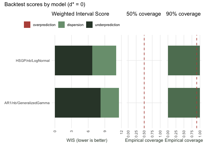

You can access these quantities directly with score

score(bt)
#>                     model      wis overprediction underprediction dispersion
#> 1       HSGP/nb/LogNormal 11.05991              0        6.722222   4.337685
#> 2 AR1/nb/GeneralizedGamma 11.54056              0        8.203704   3.336852
#>   coverage_50 coverage_90       ape      mse n
#> 1           0           1 0.7115873 1139.417 3
#> 2           0           1 0.7336961 1290.000 3

Automatic model selection

Not sure which model to pick? auto_nowcast() automates the compare-and-choose loop above: it builds a grid of candidate models sized to how much data you have, backtests them, and refits the single best one. The result is an ordinary nowcast, with the ranked comparison attached.

# Compares epidemic processes x delay families and keeps the best (default by WIS)
# here we use n_dates = 10 just as an example. Set to higher. 
# In real life this number represents how many dates are used to compare 
# the nowcasts

# Uncomment to run candidates in parallel:
# library(future)
# plan(multisession, workers = max(parallel::detectCores() - 1, 1))
auto_ncast <- auto_nowcast(dengue_tbl, n_dates = 10)
# plan(sequential)

# Get the chosen model
best_model_name(auto_ncast)
#> [1] "HSGP/nb/Dirichlet"

# Get the scores for all the models
comparison_scores(auto_ncast)
#>                      model       wis overprediction underprediction dispersion
#> 1        HSGP/nb/Dirichlet  8.295708     0.06666667        5.147778   3.081264
#> 2        HSGP/nb/LogNormal  8.448542     0.06666667        5.220000   3.161875
#> 3         AR1/nb/Dirichlet  8.512125     0.06666667        5.819444   2.626014
#> 4 HSGP/nb/GeneralizedGamma  8.624472     0.06666667        5.330000   3.227806
#> 5         AR1/nb/LogNormal  8.916250     0.05555556        5.916111   2.944583
#> 6  AR1/nb/GeneralizedGamma  8.919347     0.06666667        6.077778   2.774903
#> 7         SIR/nb/LogNormal 16.660708     0.01111111       13.270000   3.379597
#> 8         SIR/nb/Dirichlet 17.512181     0.01111111       14.362222   3.138847
#> 9  SIR/nb/GeneralizedGamma 18.083403     0.01111111       14.682778   3.389514
#>   coverage_50 coverage_90       ape      mse  n
#> 1         0.3         0.9 0.7641435  676.100 10
#> 2         0.2         0.9 0.7904566  664.600 10
#> 3         0.0         0.8 0.7887334  650.700 10
#> 4         0.1         0.9 0.7989751  738.000 10
#> 5         0.1         0.8 0.7658455  714.100 10
#> 6         0.1         0.8 0.8019557  709.425 10
#> 7         0.3         0.5 0.7541397 1467.925 10
#> 8         0.3         0.5 0.7465948 1506.100 10
#> 9         0.3         0.5 0.7537398 1514.675 10

autoplot(auto_ncast)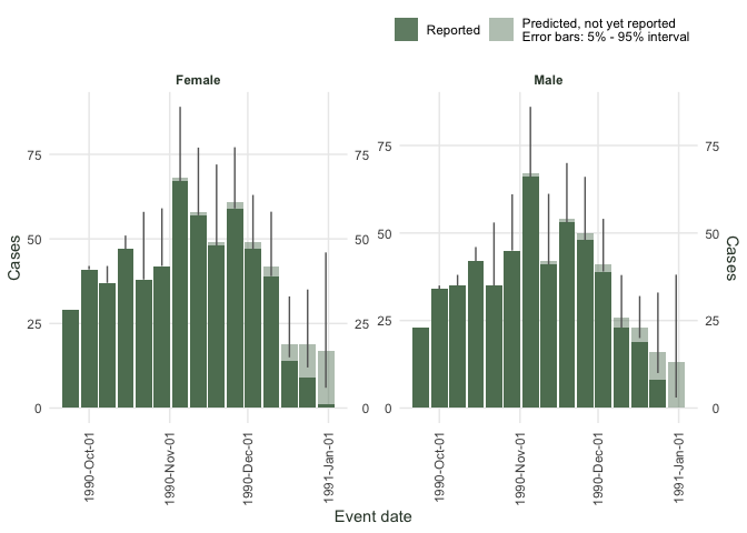

You can also feed it priors (sir = sir_epidemic(R0 = ...)), compare likelihoods (likelihood = list(nb_likelihood(), poisson_likelihood())), or add your own custom_delay() / custom_epidemic() models via models =. See the Introduction vignette for a more complete example.

Counts that can revise downward (count-cumulative data)

Some surveillance streams report a running cumulative total for each event-time that is re-reported over time and can be revised downward as well as upward — for example when a suspected case is later re-classified as negative. The FluSight influenza hospitalisation data shipped with tbl.now is one such stream. diseasenowcasting handles these with a confirmation process: attach confirmation_process() to your model() and nowcast() automatically switches to the signed-increment (Skellam / SkNB) likelihood when the data are "count-cumulative".

data(flusight, package = "tbl.now")

# Cumulative influenza hospitalisations for California, re-reported week by week
california <- flusight |>
  filter(location_name == "California", target_end_date >= as.Date("2023-10-01"))

flu_tbl <- tbl_now(
  california,
  event_date  = target_end_date,  # the epiweek being counted
  report_date = as_of,            # when that cumulative count was known
  case_count  = observation,      # cumulative admissions (can revise up OR down)
  data_type   = "count-cumulative",
  now         = as.Date("2024-01-27")
)

flu_model <- model(
  likelihood   = nb_likelihood(),
  epidemic     = ar1_epidemic(),
  delay        = lognormal_delay(),
  confirmation = confirmation_process()   # <- models the up- and down-revisions
)

flu_ncast <- nowcast(flu_tbl, flu_model, n_draws = 1000)
autoplot(flu_ncast)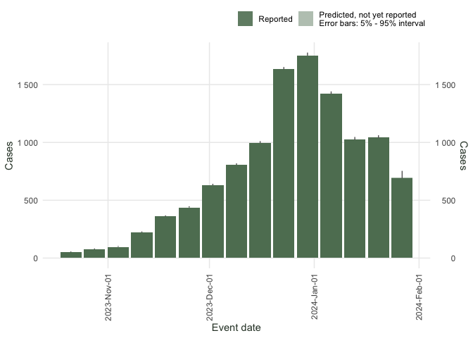

Confirmation nowcast for cumulative influenza hospitalisations in California.

The confirmation probability p — the chance a report is genuine and never retracted — is estimated with a strong data-informed prior by default; pass confirmation_process(p = 0.98) to hold it fixed, or your own beta_prior() to change the prior. For several locations at once, declare the location column as strata: a single stratified nowcast() then shares the delay and confirmation structure across locations (which is both faster and, on FluSight, sharper than a separate fit per location).

Handling extreme delays

When new data arrives, update() re-scores every incoming report against the previously fitted delay distribution and warns about anything that seems implausibly delayed. The flagged reports are available via extreme_values():

#Simulate getting new data
dengue_update <- denguedat |> 
  filter(onset_week <= as.Date("1991-01-14") & report_week <= as.Date("1991-01-14"))

# level stands for when should we flag something is an extreme delay
# level = 0.99 means delays with probability 1  - 0.99 = 0.01 are considered extreme
nc_updated <- update(ncast, new_data = dengue_update, level = 0.99)

# The model identified two extreme (very unlikely) delays of 9 and 10 weeks: 
# A human should check them based on domain knowledge and decide whether to keep
# them or to censor them. 
extreme_values(nc_updated)  
#>   delay weight mean_tail_prob cdf_prob     lpd relative_surprise direction
#> 1     9      1       0.002823 0.997177 -6.2021            0.0054      long
#> 2    10      1       0.001422 0.998578 -6.9318            0.0026      long
#>   surprise level
#> 1    delay  0.99
#> 2    delay  0.99

A complete tutorial on handling extreme delays is available at the Handling Outlier Delays with Censoring vignette.

Saving and loading a fit

Fitting can be slow, so you can save a fitted nowcast and reload it later instead of re-fitting. RTMB’s autodiff tape can’t be written to disk, so save_nowcast() stores the model(), the input tbl_now, and each fit’s parameters plus its Laplace mode and precision — all predict() needs.

save_nowcast(ncast, "dengue_nowcast.rds")

restored <- load_nowcast("dengue_nowcast.rds")
predict(restored)               # predict() / autoplot() / coef() / tidy() all work
nowcast(restored@data, restored@model)   # or re-fit from the bundled data

How it works ?

Any model() completely separates the epidemic and the delay processes allowing the user to specify the process governing each of them. When one specifies

model(
  epidemic = hsgp_epidemic(),
  delay    = generalized_gamma_delay() 
)

what is being assigned to the model are the specific delay and epidemic processes.

The image below explains the main idea: what is observed are the outcomes at a certain event_date reported (with delay) in a report_date. The processes can be analyzed separately: the epidemic process and the delay process each on their own result in a combined (coupled) observation process:

In diseasenowcasting, the nowcast_diagnostic() function plots these processes separately so you can see the reconstructed epidemic and delay processes fitted to the data:

nowcast_diagnostic(ncast)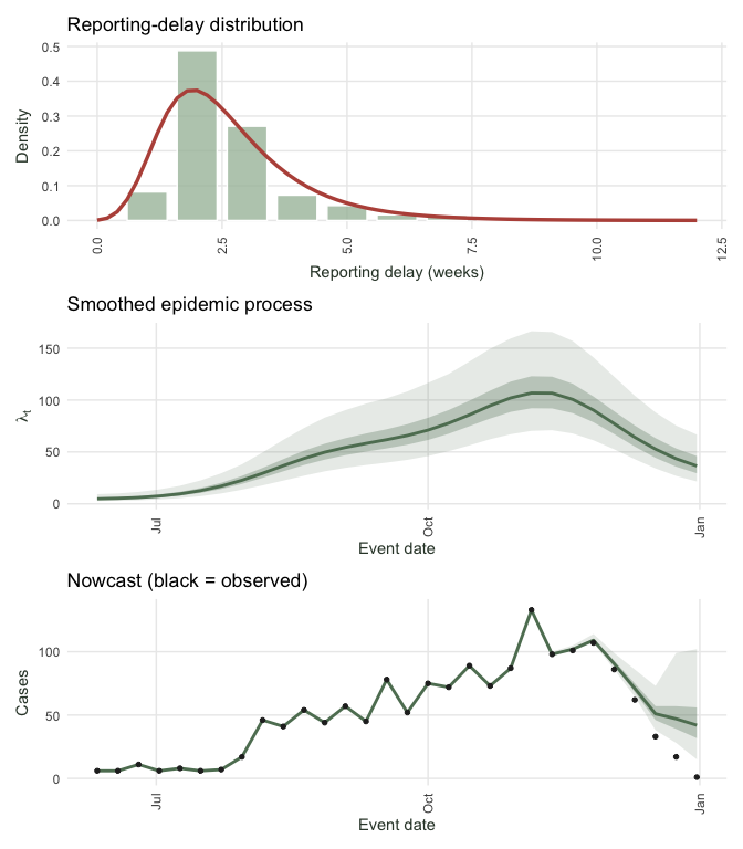

As a user, you can construct your own models within the diseasenowcasting framework via the custom_delay() and custom_epidemic() functions. You can see more in the Custom delays and epidemic processes vignette