Comparison to other methods

In this article we compare our package against the results from:

• The NobBS package.

You can go to the Comparison section directly for the comparison if you wish to skip the methods for comparing.

First we will call the libraries and generate the diseasenowcasting results.

library(diseasenowcasting, quietly = TRUE)
library(ggplot2, quietly = TRUE)
library(dplyr, quietly = TRUE)
library(lubridate, quietly = TRUE)

diseasenowcasting

In this section we will generate the estimates that will be compared against the other packages. We will operate with the following baseline model:

data(denguedat)
now   <- as.Date("1990-10-15")
ncast <- nowcast(denguedat, true_date = "onset_week", now = now,
                 report_date = "report_week", refresh = 0,
                 method = "sampling", iter = 1000,
                 seed = 27549, cores = 4, chains = 4)

and use 10 different dates in the time series codified as dates_to_test:

set.seed(645287)
dates_possible <- seq(min(denguedat$onset_week), max(denguedat$onset_week), by = "1 week")
dates_to_test  <- sample(dates_possible, size = 10) |> sort()

#We will consider only periods of at most 3 years else it makes it really slow
mindate <- min(denguedat$onset_week)

finally we will compute the nowcasts for those moments and save them into an object:

#To save the results in 
ncast_wis_table <- NULL

#The diseasenowcasting version
for (now in dates_to_test){

  #Get current date as date
  now <- as.Date(now)

  #Get new data
  new_data <- denguedat |> filter(report_week <= now & report_week >= max(now - years(3), mindate))

  #Update the model
  ncast_update  <- update(ncast, new_data = new_data, now = now)

  #Get summary
  ncast_summary <- summary(ncast_update, quantiles = c(0.025, 0.05, 0.25, 0.50, 0.75, 0.95, 0.975))

  #Save summary
  ncast_summary <- tibble(now = now, ncast_summary)

  #Keep only last observation (nowcast)
  ncast_summary <- ncast_summary |>
    mutate(horizon = as.numeric(difftime(onset_week, !!now, units="weeks"))) |>
    filter(horizon > -1)

  #Update the table
  ncast_wis_table <- rbind(ncast_wis_table, ncast_summary)

}

#Remove other columns
ncast_wis_table <- ncast_wis_table |>
  select(-sd, -median, -`50%`, -Strata_unified)

This is what it looks like:

ncast_wis_table
#> # A tibble: 10 × 10
#>    now        onset_week `2.5%`  `5%` `25%` `50%` `75%` `95%` `97.5%` horizon
#>    <date>     <date>      <dbl> <dbl> <dbl> <dbl> <dbl> <dbl>   <dbl>   <dbl>
#>  1 1990-11-12 1990-11-12   53    58    73    86.5   102  128    138         0
#>  2 1991-11-04 1991-11-04   81.0  87   109   125     142  171    182         0
#>  3 1994-06-20 1994-06-20   29.0  32    42    50      58   75     79.0       0
#>  4 1995-10-16 1995-10-16   28    32    46    56      69   88     95         0
#>  5 1999-03-08 1999-03-08   30    33    46    57      70   93    102         0
#>  6 2002-07-01 2002-07-01    1     2     4     7      12   19     23         0
#>  7 2004-02-09 2004-02-09   11    13    19    25      31   42     46         0
#>  8 2008-01-21 2008-01-21    9    11    22    31      42   63     71.0       0
#>  9 2010-05-31 2010-05-31   25    31.0  48.8  63      81  115    129         0
#> 10 2010-08-02 2010-08-02   73.0  85   131   171     223  313.   343.        0

NobBS

library(NobBS)

The usual call for the NobBS is as follows:

nbbs_cast <- NobBS(data = denguedat, units = "1 week", now = now,
                   onset_date = "onset_week", report_date = "report_week")

Here we repeat the process of analyzing multiple dates to calculate the prediction’s accuracy:

set.seed(2507284)

nobbs_wis_table <- NULL
for (now in dates_to_test){

  now <- as.Date(now)

  #Get new data
  new_data <- denguedat |> filter(report_week <= now & report_week >= max(now - years(3), mindate))

  #Update the model calculating the quantiles at 95, 90 and 50%.
  #The new Nobbs version doesn't require you to estimate three times to get quantiles
  #but I am assuming the user has the CRAN version
  nbbs_cast_95 <- NobBS(data = new_data, units = "1 week", now = now,
                     onset_date = "onset_week", report_date = "report_week",
                     specs = list(conf = 0.95))

  nbbs_cast_90 <- NobBS(data = new_data, units = "1 week", now = now,
                        onset_date = "onset_week", report_date = "report_week",
                        specs = list(conf = 0.9))

  nbbs_cast_50 <- NobBS(data = new_data, units = "1 week", now = now,
                        onset_date = "onset_week", report_date = "report_week",
                        specs = list(conf = 0.5))

  #Bind all into a single table
  nbbs_cast <- nbbs_cast_95[["estimates"]] |>
    select(estimate, lower, upper, onset_date, n.reported) |>
    rename(`97.5%` = upper, `2.5%` = lower, mean = estimate, observed = n.reported) |>
    left_join(
      nbbs_cast_50[["estimates"]] |>
      select(lower, upper, onset_date) |>
      rename(`75%` = upper, `25%` = lower), by = "onset_date"
    ) |>
    left_join(
      nbbs_cast_90[["estimates"]] |>
        select(lower, upper, onset_date) |>
        rename(`95%` = upper, `5%` = lower), by = "onset_date"
    ) |>
    mutate(horizon = as.numeric(difftime(onset_date, !!now, units="weeks"))) |>
    filter(horizon > -1) |>
    mutate(now = !!now) |>
    rename(onset_week = onset_date)

  nobbs_wis_table <- rbind(nobbs_wis_table, nbbs_cast)

}

This is what it looks like:

nobbs_wis_table
#>    mean    2.5% 97.5% onset_week observed 25% 75%     5% 95% horizon        now
#> 1   175 114.000   267 1990-11-12       16 152 203 122.00 249       0 1990-11-12
#> 2   206 141.000   293 1991-11-04       18 182 233 150.95 277       0 1991-11-04
#> 3    72  43.000   114 1994-06-20        5  61  84  47.00 107       0 1994-06-20
#> 4    51  26.975    93 1995-10-16        3  41  63  30.00  84       0 1995-10-16
#> 5    47  25.000    81 1999-03-08        1  38  57  28.00  74       0 1999-03-08
#> 6     5   1.000    14 2002-07-01       NA   3   8   1.00  12       0 2002-07-01
#> 7    28  13.000    52 2004-02-09        2  22  35  15.00  47       0 2004-02-09
#> 8    21   8.000    44 2008-01-21       NA  15  27   9.00  39       0 2008-01-21
#> 9    66  34.000   117 2010-05-31        1  53  81  38.00 108       0 2010-05-31
#> 10  477 278.000   787 2010-08-02        6 399 566 305.00 727       0 2010-08-02

Comparison

model_table <- nobbs_wis_table |> 
  mutate(method = "NoBbs") |> 
  rename(`50%` = mean) |>  #The point estimate for scoring utils
  bind_rows(ncast_wis_table |> mutate(method = "diseasenowcasting"))

We use the scoringutils library to calculate the weighted interval scoring:

library(scoringutils, quietly = TRUE)
library(tidyr)
library(stringr)

summary_table <- model_table |> 
    mutate(observed = replace_na(observed, 0)) |> 
    pivot_longer(cols = ends_with("%"), names_to = 'quantile_level', values_to = 'predicted') |>
    mutate(quantile_level = as.numeric(str_remove_all(quantile_level, "\\%"))/100)  |>
    as_forecast_quantile() |>
    score() |>
    summarise_scores(by = c("horizon","method","now"))

And format for presenting

wis_table <- summary_table |> 
  pivot_wider(id_cols = c("horizon","now"), names_from = "method", values_from = "wis") |> 
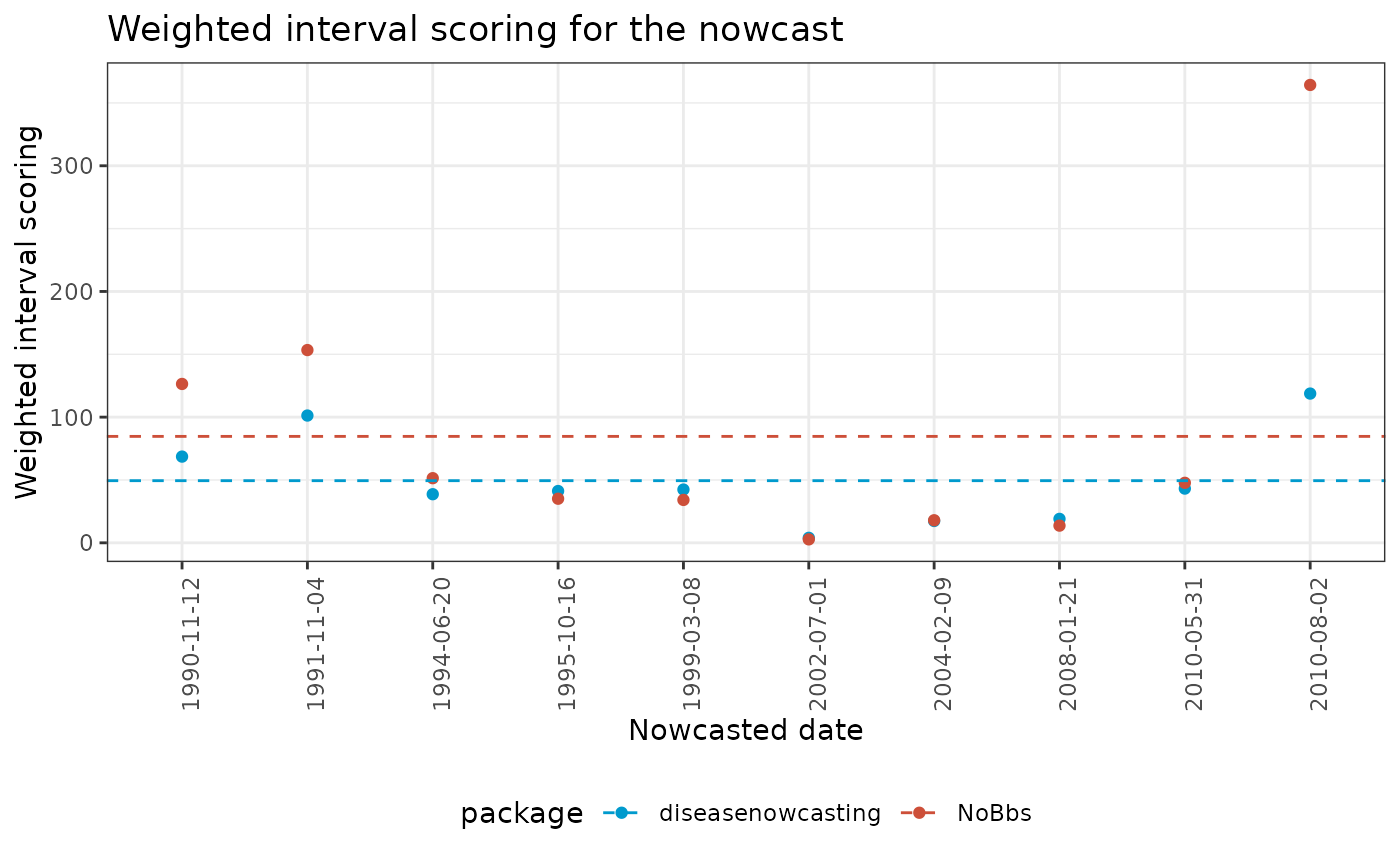
  mutate(nowcat = factor(now, ordered = TRUE))

Finally the results show that diseasenowcasting is either close to NoBbs or performs better than NoBbs:

ggplot(wis_table) +
  geom_point(aes(x = nowcat, y = diseasenowcasting, color = "diseasenowcasting")) + 
  geom_point(aes(x = nowcat, y = NoBbs, color = "NoBbs")) + 
  geom_hline(aes(yintercept = mean(NoBbs), color = "NoBbs"), linetype = "dashed") +
  geom_hline(aes(yintercept = mean(diseasenowcasting), color = "diseasenowcasting"), linetype = "dashed") +
  theme_bw() +
  labs(
    x = "Nowcasted date",
    y = "Weighted interval scoring",
    title = "Weighted interval scoring for the nowcast"
  ) +
  theme(
    legend.position = "bottom",
    axis.text.x = element_text(angle = 90, hjust = 0.5, vjust = 1)
  ) +
  scale_color_manual("package", values = c("deepskyblue3","tomato3"))