Handling Outlier Delays with Censoring

diseasenowcasting team

set.seed(248675)
library(diseasenowcasting)
library(tbl.now)
library(dplyr)
library(ggplot2)

TL; DR

In general the workflow is:

1. Fit a nowcast.

2. When new data arrives use update() to get warnings about extreme values.

3. A human with domain-knowledge identifies which ones correspond to outliers and which correspond to true values.

4. The censor_delays_above() function turns extreme delays into upper bounds.

5. Model is re-updated using the censored data consequently improving the delay distribution.

6. Backtest to verify the fit improved.

The problem: an extreme delay

Real surveillance data occasionally contains reports with extreme reporting delays. This can be due to typos, healthcare-system hurdles or other issues not related to the disease’s natural evolution. In Colombia’s COVID-19 data (covid_colombia) the bulk of reports arrive within a week or two, but a handful take more than 100 days:

data(covid_colombia)

tbl_covid <- covid_colombia |> 
  tbl_now(event_date  = notification_date,
          case_count  = n,
          data_type   = "count-incidence",
          report_date = diagnosis_date,
          t_effects   = temporal_effects(day_of_week = TRUE))

summary(tbl_covid$.delay)
#>    Min. 1st Qu.  Median    Mean 3rd Qu.    Max. 
#>     0.0     4.0    10.0    11.6    17.0   330.0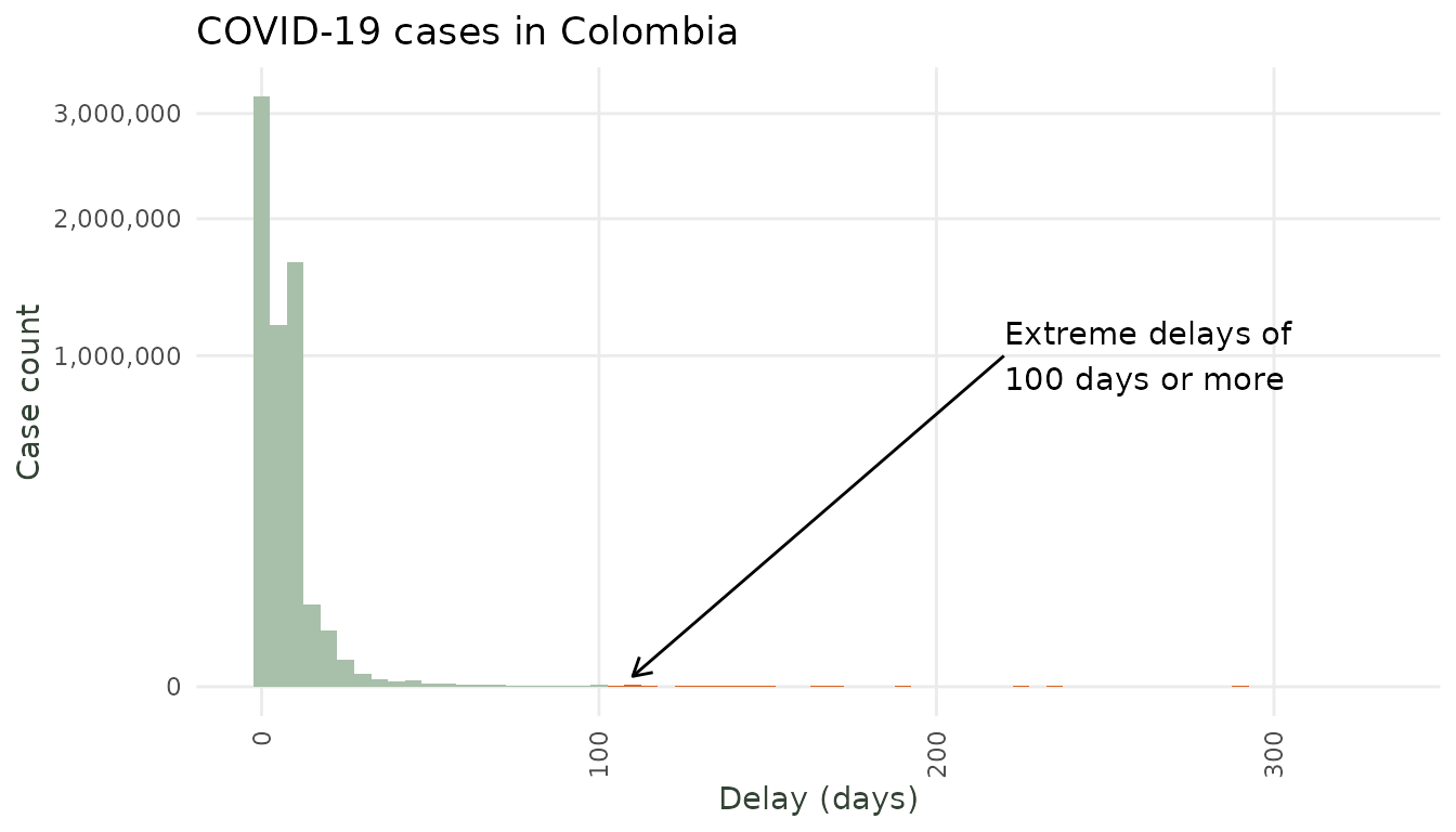

Reporting-delay distribution of COVID-19 Colombia (extremes exagerated for illustration purposes). A few reports arrive hundreds of days late.

When a parametric delay model (log-normal, gamma, …) is fit to data containing such an outlier, the extreme value drags the estimated delay distribution to the right. The model then believes delays are longer than they really are, thus inflating the most recent nowcasts.

The diseasenowcasting framework offers a fix. It treats such reports as right-censored. Instead of telling the model “this case had delay exactly 330”, it tells it only “this case arrived by delay 330” (i.e. its delay of 330 is an upper bound for the true delay).

In what follows we explain how to use the model to automatically detect extreme delays and how to inform the model so that predictions are improved.

1) Fit a model

The first step for a model to learn about extreme delays is to have an initial model with historical data so that it learns what the usual distribution is. In this case we’ll work with an early-pandemic window and fit a nowcast(). To play out the “new data arrives” story we first fit on the reports available at an early date (2020-08-31):

#Initial data
initial_tbl <- tbl_covid |> 
  filter(
    notification_date <= as.Date("2020-08-31") & 
    diagnosis_date <= as.Date("2020-08-31")) |> 
  change_now() #Update the "now" of the nowcast to the latest date

We then fit a nowcast to this data (in this example, the next day, 2020-09-01):

initial_ncast <- nowcast(initial_tbl)

2) Update the model

We can then get new data:

new_data_tbl <- tbl_covid |> 
  filter(
    notification_date <= as.Date("2020-09-01") & 
    diagnosis_date <= as.Date("2020-09-01")) |> 
  change_now()

and update() the model. This will automatically score the new data against the old fit and warn that something is amiss:

nc_updated <- update(initial_ncast, new_data_tbl)
#> Warning: ! Surprising reporting delay of 114 days (1 report): longer than the model
#>   expects (P(D >= d) = 0.00051).
#> ! Surprising reporting delay of 112 days (1 report): longer than the model
#>   expects (P(D >= d) = 0.00055).
#> ! Surprising reporting delay of 99 days (1 report): longer than the model
#>   expects (P(D >= d) = 0.00087).
#> ℹ If these are outliers, treat them as censored with `censor_delays_above()`
#>   and re-fit.
#> ℹ See all flagged delays with `extreme_values(nc)`.

The warning tells us exactly what was unexpected (reporting delays far longer than usual). The full table is available via extreme_values():

extreme_values(nc_updated)
#>   delay weight mean_tail_prob cdf_prob      lpd relative_surprise direction
#> 1    99      1       0.000870 0.999130 -10.3354             3e-04      long
#> 2   112      1       0.000547 0.999453 -10.8867             2e-04      long
#> 3   114      1       0.000511 0.999489 -10.9672             1e-04      long
#>   surprise level
#> 1    delay  0.99
#> 2    delay  0.99
#> 3    delay  0.99

The mean_tail_prob expressess the probability of observing such a value, The cdf_prob the probability of lying below that value. Variable level shows the level of certainty to qualify something as an outlier (default = 0.99) and can be modified in update(..., level = 0.95). Column delay corresponds to the observed delay and weight corresponds to how many times it was observed. Finally lpd stands for the log pointwise predictive density value.

3) Censor the outliers and re-fit

We follow the warning’s advice: we flag as censored every report whose delay exceeds a sensible bound (here 99 days as reported by extreme_values()). The function censor_delays_above() works by setting .is_censored = TRUE in the tbl_now for reports greater than the max_delay. Extreme delays are thus turned into upper bounds. The nowcast() then reads the .is_censored flag automatically.

new_data_tbl_censored <- censor_delays_above(new_data_tbl, max_delay = 99)

#Adds column `.is_censored`:
new_data_tbl_censored

#> # A tibble:  7,798 × 8
#> # Data type: "count-incidence"
#> # Frequency: Event: `days` | Report: `days`
#>    .is_censored  notification_date diagnosis_date sex          n .event_num
#>    <lgl>         <date>            <date>         <chr>    <int>      <dbl>
#>    [is_censored] [event_date]      [report_date]  [...]  [cases]      [...]
#>  1 FALSE         2020-03-02        2020-03-06     Female       1          0
#>  2 FALSE         2020-03-03        2020-03-14     Female       1          1
#>  3 FALSE         2020-03-06        2020-03-09     Male         1          4
#>  4 FALSE         2020-03-07        2020-03-09     Female       1          5
#>  5 FALSE         2020-03-08        2020-03-11     Female       2          6
#>  6 FALSE         2020-03-09        2020-03-11     Female       1          7
#>  7 FALSE         2020-03-09        2020-03-11     Male         2          7
#>  8 FALSE         2020-03-10        2020-03-11     Female       1          8
#>  9 FALSE         2020-03-10        2020-03-12     Female       2          8
#> 10 FALSE         2020-03-10        2020-03-13     Male         1          8
#> # ────────────────────────────────────────────────────────────────────────────────
#> # Now: 2020-09-01 | Event date: "notification_date" | Report date:
#> # "diagnosis_date"
#> # Right-censored indicator: ".is_censored"
#> # T. effects (lazy): [event_date] day_of_week
#> # ────────────────────────────────────────────────────────────────────────────────
#> # ℹ 7,788 more rows
#> # ℹ 2 more variables: .report_num <dbl>, .delay <dbl>

We refit but this time using the censored data:

nc_updated_censored <- update(initial_ncast, new_data_tbl_censored)

The fitted values change once the outliers are no longer taken literally.

#Previous
coef(nc_updated)
#>     delay_mu  delay_sigma       phi_nb mu_intercept log_gp_alpha   log_gp_ell 
#>    2.2038885    9.4014684    0.1163241    7.6319443    1.2491609   -1.6613317

#Updated
coef(nc_updated_censored)
#>     delay_mu  delay_sigma       phi_nb mu_intercept log_gp_alpha   log_gp_ell 
#>   2.21249391   9.39874394   0.07725975   7.65454383   1.23644661  -1.63696766

Which also affects predictions:

#Previous
pred_previous <- predict(nc_updated) 
summary(pred_previous) |> tail(6)
#>         mean  median       sd      mad     q2.5      q5    q10     q25     q50
#> 179 10694.38 10202.0 2525.602 1999.286 7298.875 7722.60 8170.4 9003.25 10202.0
#> 180 11044.44 10541.5 2753.292 2278.015 7164.925 7549.70 8164.9 9216.75 10541.5
#> 181 10766.30 10208.5 3308.333 2589.361 6085.425 6562.80 7296.4 8657.00 10208.5
#> 182 10596.68  9971.0 3738.150 3088.997 5263.875 5877.65 6580.8 8134.75  9971.0
#> 183 12537.80 11967.5 3945.864 3450.010 6641.750 7303.90 8241.4 9812.25 11967.5
#> 184 12239.32 11696.5 4210.472 3697.604 5496.275 6451.40 7582.3 9492.75 11696.5
#>          q75     q90      q95    q97.5 .event_num
#> 179 11811.00 13767.7 15241.10 16647.15        178
#> 180 12341.50 14464.3 16057.75 17662.00        179
#> 181 12261.25 14508.5 16688.35 18763.27        180
#> 182 12366.00 15045.5 17181.30 19415.30        181
#> 183 14551.25 17436.4 19613.40 22166.62        182
#> 184 14515.50 17494.0 19793.55 21752.22        183

#Updated
pred_censored <- predict(nc_updated_censored)
summary(pred_censored) |> tail(6)
#>         mean  median       sd      mad     q2.5      q5    q10     q25     q50
#> 179 10718.00 10238.5 2400.787 1929.604 7345.550 7744.95 8176.3 9107.00 10238.5
#> 180 11225.55 10683.5 2956.454 2446.290 7121.725 7622.90 8138.5 9212.25 10683.5
#> 181 10836.18 10305.5 3094.822 2871.055 6155.900 6692.35 7459.9 8652.75 10305.5
#> 182 10870.68 10148.0 3748.603 3274.322 5500.950 6123.15 6883.6 8243.50 10148.0
#> 183 12600.18 12041.0 4071.793 3629.405 6577.825 7185.80 8099.4 9840.50 12041.0
#> 184 12339.74 11799.0 4365.927 3799.904 5565.925 6421.65 7618.6 9373.75 11799.0
#>          q75     q90      q95    q97.5 .event_num
#> 179 11832.00 13970.7 15453.65 16619.03        178
#> 180 12632.00 14748.2 16619.90 18734.40        179
#> 181 12552.50 14827.4 16672.00 18195.77        180
#> 182 12803.25 15822.6 17725.55 19685.60        181
#> 183 14787.50 17702.7 19935.70 22050.37        182
#> 184 14546.75 17657.5 20027.95 22402.47        183

4) Does it nowcast better? Backtest

Finally we check if controlling the extreme values actually improves accuracy. We backtest the same model on the plain data (new_data_tbl) and on the censored data (new_data_tbl_censored) across a set of dates, scoring the most recent nowcast (d^* = 0) against the eventual truth with the Weighted Interval Score (WIS; lower is better) and coverage (closer to the expected coverage the better).

#dates to backtest
eval_dates <- as.Date(c("2020-04-15", "2020-05-01", 
                        "2020-05-15", "2020-06-01"))

#Backtest each model on the same dates
bt_plain   <- backtest(new_data_tbl, dates = eval_dates)
bt_cens    <- backtest(new_data_tbl_censored, dates = eval_dates)

rbind(
  plain    = score(bt_plain, report = F)[,c("wis","coverage_50","coverage_90")],
  censored = score(bt_cens,  report = F)[,c("wis","coverage_50","coverage_90")]
)
#>               wis coverage_50 coverage_90
#> plain    211.3629         0.5         0.5
#> censored 206.6438         0.5         0.5

Censoring these outlier delays result in a lower (better) WIS and a similar coverage in this example. Though in a real test we would need to backtest through more dates to reach a conclusion.

Summary – fit -> update -> identify outliers -> censor -> refit loop

In general the workflow is:

1. Fit a nowcast.

2. New data arrives -> update() scores it and warns about potential outliers.

3. Manually identify which ones correspond to outliers and which correspond to true values. This has to be done by a human as no automated system will know when something flagged as noise is real.

4. Use censor_delays_above(tn, bound) turning the delays into an upper bound. Or modify the tbl_now directly (column is_censored)

5. Re-fit -> the delay distribution is no longer distorted.

6. Backtest to verify the fit improved.