Custom Delays and Epidemic Processes

diseasenowcasting team

diseasenowcasting is a model-agnostic nowcasting framework. A nowcast here is built from three pieces:

• A likelihood,

• An epidemic process, and

• A reporting-delay distribution.

You can either pick a built-in for the epidemic and the delay or supply your own.

This vignette shows how to extend the epidemic and delay processes to custom models via two examples based on a real dataset:

• A custom delay distribution (Weibull), fit to weekly dengue surveillance (tbl.now::denguedat); and

• a custom epidemic process (hand-written SIR model), fit to the 2022 mpox outbreak (tbl.now::mpoxdat).

The one rule: RTMB

To fit, the package needs the gradient of the likelihood with respect to the parameters. It gets this automatically via automatic differentiation (AD) through the RTMB) package. If you are unfamiliar with it here are some basic rules:

1. Write your function in plain arithmetic. Use +, -, *, /, exp, log, sqrt, abs, sum, cumsum, pnorm, pgamma, and fixed-length for loops (loops that depend on sample size or time but not on a parameter).

2. Avoid conditioning on parameters Never use if/ifelse on a parameter value nor pmax/pmin on parameters. There are always work around such as using (x + abs(x))/2 for pmax(x, 0).

3. Don’t use random draws nor external solvers (e.g. for differential equations or optimization). deSolve can be used via the additional RTMBode library.

Note Each extension has a validator (validate_custom_delay(), validate_custom_epidemic()). It checks your function for possible errors. The validator is not perfect and might raise false-positive flags (i.e. functions that do work on RTMB might crash the validator). So if you know what you are doing feel free to ignore it.

set.seed(26378)
library(diseasenowcasting)
library(tbl.now)
library(RTMB) # <--------- REQUIRED for custom components 
library(ggplot2)
library(dplyr)

1. Custom delay: Weibull

The data

denguedat is a weekly dengue line-list from Puerto Rico (onset_week, report_week). We take one season and build a tbl_now, which carries the two time indices the nowcast needs:

#Get just one season for making the example fast
dengue_season <- denguedat |> 
  filter(report_week  <= as.Date("1991-06-01") & 
           onset_week <= as.Date("1991-06-01"))

#Construct the tbl_now
dengue_tn <- tbl_now(dengue_season,
                     event_date  = onset_week,
                     report_date = report_week,
                     data_type   = "linelist",
                     verbose     = FALSE)

The custom part: a Weibull delay

You describe the delay through its cumulative distribution function (CDF) F(d). Each piece is written as a function of a parameter vector named theta that returns a function of the delay d.

Note theta represents a transformation of the parameters so that they are unconstrained (\theta \in \mathbb{R}^k. It might not be equal to the ‘usual’ parameters as we explain below.

Argument	Meaning	Weibull form	Required?
cdf(theta)	returns function(d) = F(d) = \Pr(\text{delay} \le d)	1 - \exp(-(d/\lambda)^k)	yes
log_cdf(theta)	returns function(d) = \log F(d)	defaults to \log(\text{cdf})	no
log_survival(theta)	returns function(d) = \log(1 - F(d))	-(d/\lambda)^k	no

Only cdf is required; log_cdf and log_survival default to the obvious transforms of cdf. It is worth supplying log_survival and log_cdf explicitly for numerical stability. For example, the default log(1 - cdf) loses precision as F \to 1, whereas for the Weibull log_survival = -(d/\lambda)^k is exact. We work on the log scale (theta[1] = log k, theta[2] = log lambda) so the optimizer is unconstrained.

weibull_cdf <- function(theta) {
  shape <- exp(theta[1])   # k > 0
  scale <- exp(theta[2])   # lambda > 0
  function(d) 1 - exp(-(d / scale)^shape)
}

weibull_log_survival <- function(theta) {
  shape <- exp(theta[1])   # k > 0
  scale <- exp(theta[2])   # lambda > 0
  function(d) -(d / scale)^shape         # exact log(1 - F), stable in the tail
}

Pass them to custom_delay(). The arguments:

• cdf (and optionally log_cdf, log_survival) — the functions above.
• priors — a list with one entry per parameter, in theta order. Each entry is either a prior (a free parameter, estimated) or a single number (fixed).
• name, param_names, inits — labels and (unconstrained-scale) starting values.

weibull_delay <- custom_delay(
  cdf          = weibull_cdf,
  log_survival = weibull_log_survival,
  priors       = list(normal_prior(0, 1), normal_prior(log(3), 1)),
  name         = "Weibull",
  param_names  = c("log_shape", "log_scale"),
  inits        = c(0, log(3))
)
validate_custom_delay(weibull_delay)

Fit it (and a built-in to compare against)

The Generalized Gamma reduces exactly to a Weibull when its shape parameter Q = 1, so generalized_gamma_delay(Q = 1) is a perfect built-in cross-check for our custom delay:

#Custom delay
nc_weibull  <- nowcast(dengue_tn,
                       model(likelihood = nb_likelihood(),
                             epidemic   =  ar1_epidemic(), 
                             delay      = weibull_delay),
                       temporal_effects = "none")

#Using the Generalized Gamma from the package
nc_gengamma <- nowcast(dengue_tn,
                       model(likelihood = nb_likelihood(), 
                             epidemic   = ar1_epidemic(), 
                             delay      = generalized_gamma_delay(Q = 1)),
                       temporal_effects = "none")

The two coincide confirming the custom delay matches a known distribution:

Show plotting code

delay_grid <- seq(0.5, 20, by = 0.5)
pmf <- function(shape, scale)
  stats::pweibull(delay_grid + 0.5, shape, scale) -
  stats::pweibull(pmax(0, delay_grid - 0.5), shape, scale)

#Get the fitgted parameyters
theta_w <- as.numeric(nc_weibull@fits[[1]]$parList$custom_delay_params)
mu_g    <- nc_gengamma@fits[[1]]$reconstruct$delay_mu
sig_g   <- nc_gengamma@fits[[1]]$reconstruct$delay_sigma

compare_df <- rbind(
  data.frame(delay = delay_grid, p = pmf(exp(theta_w[1]), exp(theta_w[2])), model = "Custom Weibull"),
  data.frame(delay = delay_grid, p = pmf(1 / sig_g, exp(mu_g)),            model = "GenGamma (Q=1)")
)
ggplot(compare_df, aes(delay, p, colour = model, linetype = model)) +
  geom_line(linewidth = 1.1) +
  scale_colour_manual(values = c("Custom Weibull" = "#2166AC", "GenGamma (Q=1)" = "#D6604D")) +
  labs(x = "Reporting delay (weeks)", y = "Probability mass",
       title = "Custom Weibull vs. built-in GenGamma(Q = 1)", colour = NULL, linetype = NULL) +
  theme_minimal(base_size = 13) + theme(legend.position = "bottom")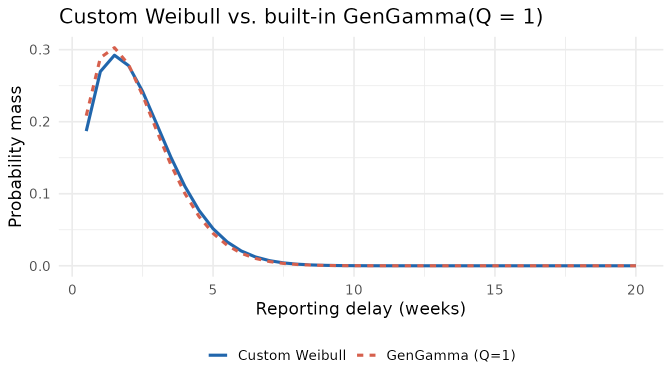

Fitted reporting-delay distribution: custom Weibull vs. the built-in GenGamma(Q=1), which is algebraically the same Weibull.

And the nowcast itself, using the custom delay:

autoplot(predict(nc_weibull, seed = 246))

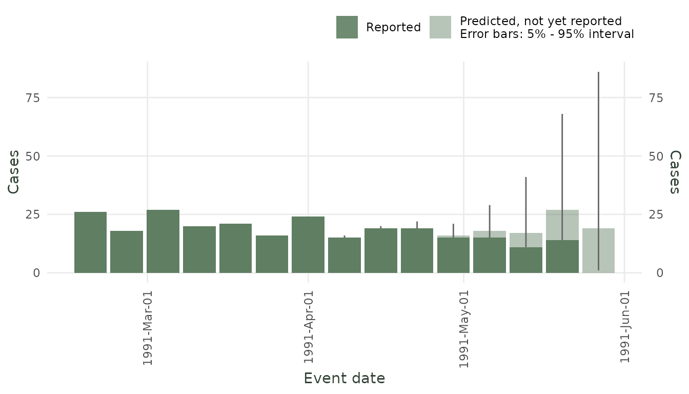
Dengue nowcast with the custom Weibull delay (median + 50/90% intervals).

2. Custom epidemic: different SIR

A custom epidemic is just one function intensity_fn(theta) that returns the log expected-incidence matrix log_mean[n_time × n_strata]. How you generate it (regression, random walk, ODE, …) is up to you.

The data

mpoxdat is daily count data from the 2022 US mpox outbreak. We pool the race strata into one series and build a tbl_now:

mpox_tn <- tbl_now(mpoxdat,
                   event_date  = dx_date,
                   report_date = dx_report_date,
                   case_count  = n,
                   data_type   = "count-incidence",
                   verbose     = FALSE,
                   now         = as.Date("2022/09/01"))

The SIR loop runs over every event-time, so we need max_time (the number of event-times the model spans) before writing the function. infer_max_time() reads it off the data:

max_time <- infer_max_time(mpox_tn)

The custom part: an SIR epidemic

This is the code that matters. A discrete-time SIR with susceptibles (S) and infectious (I) evolving on a daily basis. The modelled incidence is the new infections beta·S·I/N. The parameters (R0, gamma, I0) are again on the log scale (unconstrained).

sir_intensity_fn <- function(theta) {
  #Assigning in a for loop a vector requires this:
  `[<-`     <- RTMB::ADoverload("[<-")         
  
  #We define R0, gamma and I0 as the parameters we are adjusting:
  R0        <- exp(theta[1])   #Basic reproductive number
  gamma     <- exp(theta[2])   #1 / infectious rate
  I0        <- exp(theta[3])   #Initial infected
  
  #The total size of the population is constant:
  N         <- 1e5
  
  #Initial values for S and I
  S         <- N - I0
  I         <- I0
  
  #Beta (for force of infection)
  beta      <- R0 * gamma / N
  
  #Empty vector where we'll store the incidence. Has to be instantiated in RTMB
  incidence <- numeric(max_time)

  #Only loops that don't depend on parameters are allowed.
  #Here we loop through a constant (time) which is valid
  for (t in seq_len(max_time)) {

    new_inf      <-  beta * S * I
    incidence[t] <- new_inf

    #Rest of the model
    S <- S - new_inf
    I <- I + new_inf - gamma * I
  }
  # log of pmax(incidence, 0), AD-safe, guarding log(0):
  matrix(log((incidence + abs(incidence)) * 0.5 + 1e-8), max_time, 1L)
}

Wrap it in custom_epidemic() (same argument shape as custom_delay()):

custom_sir_epidemic <- custom_epidemic(
  intensity_fn = sir_intensity_fn,
  priors       = list(normal_prior(log(1.5), 0.4),   # log R0
                      normal_prior(log(0.1), 0.3),   # log gamma
                      normal_prior(log(5),   1.0)),  # log I0
  name         = "SIR",
  param_names  = c("log_R0", "log_gamma", "log_I0"),
  inits        = c(log(1.5), log(0.1), log(5))
)
validate_custom_epidemic(custom_sir_epidemic)

Fit it

nc_sir_custom  <- nowcast(mpox_tn,
                          model(likelihood = nb_likelihood(), 
                                epidemic   = custom_sir_epidemic, 
                                delay      = lognormal_delay()),
                          temporal_effects = "none")

And observe the results:

autoplot(nc_sir_custom)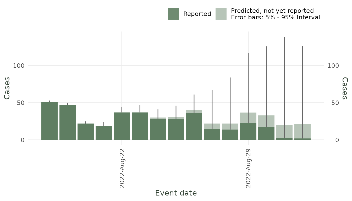

mpox nowcast with the custom SIR epidemic (median + 50/90% intervals).

3. Summary: Tips for writing your own component

1. Parametrize on the unconstrained scale. Use exp(theta[i]) for positive quantities, plogis(theta[i]) for probabilities. Give the initial values inits on that same scale.
2. A custom epidemic represents the whole log_mean. Include any baseline level. Use all covariates you need. Nothing (no intercept, no covariates) is added on top after you set it.
3. Know max_time first if your function loops over time. infer_max_time(tn) gives the number of event-times the model spans.
4. Use [<- to accumulate vectors Use `[<-` <- RTMB::ADoverload("[<-") only when a loop must fill a pre-allocated vector (e.g. an ODE).
5. Guard log of near-zero values The log((x + abs(x)) * 0.5 + 1e-8) we used is a numerically-safe way to calculate the maximum and avoid log(0).
6. Validate before fitting — validate_custom_delay() / validate_custom_epidemic() help catch code errors early.
7. Use other packages, the RTMBode package offers an adaptive/stiff solver that plugs into RTMB. Might be helpful for more complicated models.

4. Advanced: A differential equations epidemic process

Here we write the epidemic as a continuous-time SIR ordinary differential equation and let a proper solver integrate it. The RTMBode package provides a deSolve-style ode() that is differentiable through RTMB (it supplies the adjoint), so there is no need to hand-roll an integrator such as Runge–Kutta.

The SIR system is

\frac{dS}{dt} = -\beta\,S\,I, \qquad \frac{dI}{dt} = \beta\,S\,I - \gamma\,I, \qquad \beta = \frac{R_0\,\gamma}{N},

and the daily incidence is the number of new infections within each day. We obtain it by adding a cumulative-infection compartment C with dC/dt = \beta\,S\,I; the per-day incidence is then diff(C) across the day boundaries 0, 1, \dots, \texttt{max\_time}.

RTMBode is an optional dependency; install it from the kaskr r-universe:

install.packages("RTMBode", repos = "https://kaskr.r-universe.dev")

sir_ode_fn <- function(theta) {
  #We define R0, gamma and I0 as the parameters we are adjusting (log scale,
  #so they are always positive):
  R0    <- exp(theta[1])   #Basic reproductive number
  gamma <- exp(theta[2])   #Recovery rate (1 / infectious period)
  I0    <- exp(theta[3])   #Initial infected

  #The total population is constant; beta is the transmission rate:
  N     <- 1e5
  beta  <- R0 * gamma / N

  #The SIR right-hand side, deSolve-style: a function of (time, state, parms)
  #returning the derivatives. We add a compartment C that ACCUMULATES new
  #infections, so the daily incidence is simply diff(C).
  sir_rhs <- function(time, state, parms) {
    with(as.list(c(state, parms)), {
      infection <- beta * S * I
      list(c(-infection,                # dS/dt
              infection - gamma * I,    # dI/dt
              infection))               # dC/dt  (cumulative infections)
    })
  }

  #RTMBode::ode is a deSolve-compatible solver that is differentiable through
  #RTMB (it supplies the adjoint), so we let it integrate the system instead of
  #hand-rolling RK4. Solve at the day boundaries 0, 1, ..., max_time:
  solution  <- RTMBode::ode(
    y     = c(S = N - I0, I = I0, C = 0),
    times = seq.int(0L, max_time),
    func  = sir_rhs,
    parms = c(beta = beta, gamma = gamma)
  )
  incidence <- diff(solution[, "C"])     # new infections within each day

  # log of pmax(incidence, 0), AD-safe, guarding log(0):
  matrix(log((incidence + abs(incidence)) * 0.5 + 1e-8), max_time, 1L)
}

The wrapping and fitting are exactly as before:

sir_ode_epidemic <- custom_epidemic(
  intensity_fn = sir_ode_fn,
  priors       = list(normal_prior(log(1.5), 0.4),
                      normal_prior(log(0.1), 0.3),
                      normal_prior(log(5),   1.0)),
  name         = "SIR-ODE",
  param_names  = c("log_R0", "log_gamma", "log_I0"),
  inits        = c(log(1.5), log(0.1), log(5))
)

#Check the custom model
validate_custom_epidemic(sir_ode_epidemic)

#Do the nowcast
nc_ode <- nowcast(mpox_tn,
                  model(nb_likelihood(), sir_ode_epidemic, lognormal_delay()),
                  temporal_effects = "none")

nowcast_diagnostic(nc_ode)