library(tidyverse)
library(tidymodels)
library(ggfortify) # autoplot para diagnósticos
library(rstanarm) # para bayesiana
library(poissonreg) # modelo Poisson

# Siempre que uses tidymodels
tidymodels_prefer()12 Regresiones (parte 2)
Advertencia
Si no lo has leído aún ve la parte 1 de regresiones
12.1 Paquetes y datos a utilizar
A lo largo de esta sección usaremos los siguientes paquetes:
En general usaremos la filosofía tidymodels para combinar los resultados con el tidyverse. Si quieres saber más de tidymodels te recomiendo checar su libro o su página web.
13 Modelos lineales generalizados
13.1 Regresión Poisson (conteo)
Anteriormente planteamos el modelo
\[ y \sim \textrm{Normal}(\beta_0 + \beta_1 x, \sigma^2) \]
podemos cambiar la distribución normal por una Poisson si tenemos datos de conteo, por ejemplo:
\[ y \sim \textrm{Poisson}(\beta_0 + \beta_1 x) \]
¡Y ya tenemos una regresión Poisson! Ésta no es la clásica pues es bien difícil de controlar numéricamente. La Poisson clásica tiene una exponencial adentro:
\[ y \sim \textrm{Poisson}\big(\exp(\beta_0 + \beta_1 x)\big) \]
Usaremos esta última para los modelos. Para ello nos apoyaremos del engine de glm (por generalized linear model)
Para los datos usaremos la información de Generalized Linear Models for Cross-Classified Data from the WFS. World Fertility Survey Technical Bulletins . Podemos leerlos como sigue:
# Copia local de los datos de ceb.dat de https://data.princeton.edu/wws509/datasets/
niños <- read_table("datasets/niños.txt", skip = 1, col_names = F)
colnames(niños) <- c("Fila", "dur", "res", "educ", "mean", "var", "n", "y")
niños <- niños %>% mutate(y = round(y))
La base contiene la dur la duración del matrimonio, res la residencia (suva, urbano y rural), el nivel educativo educ, la media y la varianza del número de niños nacidos y n la cantidad de mujeres en cada grupo. La variable y contiene el producto de mean*n para obtener el total de niños nacidos para todas las mujeres en cada grupo.
Podemos especificar fácilmente un modelo Poisson para los conteos:
modelo_poisson <- poisson_reg() %>%
  set_engine("glm") %>%
  fit(y ~ educ, data = niños)
podemos obtener el summary:
modelo_poisson %>%
  extract_fit_engine() %>%
  summary()
Call:
stats::glm(formula = y ~ educ, family = stats::poisson, data = data)

Coefficients:
            Estimate Std. Error z value Pr(>|z|)
(Intercept)  5.38780    0.01594  338.06  < 2e-16 ***
educnone     0.16257    0.02168    7.50 6.39e-14 ***
educsec+    -2.13937    0.05178  -41.32  < 2e-16 ***
educupper   -0.88738    0.02951  -30.07  < 2e-16 ***
---
Signif. codes:  0 '***' 0.001 '**' 0.01 '*' 0.05 '.' 0.1 ' ' 1

(Dispersion parameter for poisson family taken to be 1)

    Null deviance: 13735.6  on 69  degrees of freedom
Residual deviance:  9076.8  on 66  degrees of freedom
AIC: 9514.3

Number of Fisher Scoring iterations: 5
o crear un tibble:
modelo_poisson %>%
  extract_fit_engine() %>%
  tidy()
# A tibble: 4 × 5
term estimate std.error statistic p.value
<chr> <dbl> <dbl> <dbl> <dbl>
1 (Intercept) 5.39 0.0159 338. 0
2 educnone 0.163 0.0217 7.50 6.39e- 14
3 educsec+ -2.14 0.0518 -41.3 0
4 educupper -0.887 0.0295 -30.1 1.22e-198o también podemos ajustarlo de manera bayesiana:
poisson_reg() %>%
  set_engine("stan") %>%
  fit(y ~ educ, data = niños) %>%
  extract_fit_engine() %>%
  summary()
Podemos agregar más factores a nuestra regresión. Para ello vale la pena recordar las fórmulas de R:
| Fórmula | Significado |
|---|---|
1 |
El intercepto |
+x |
Agregar la variable x a la regresión |
-x |
Quitar la variable x de la regresión |
x1:x2 |
Interacción entre x1 y x2 |
x1*x2 |
Cruzamiento es lo mismo que poner x1 + x2 + x1:x2 |
I() |
Se utiliza para realizar operaciones aritméticas adentro. Por ejemplo generar una variable que sea x1+ x2 haciendo I(x1 + x2) |
(x | grupo) |
Modelos mixtos donde la pendiente de x depende del grupo (efectos aleatorios) |
En nuestro modelo podemos incluir otras variables (digamos la residencia) agregándolas con suma:
poisson_reg() %>%
  set_engine("glm") %>%
  fit(y ~ educ + res, data = niños) %>%
  extract_fit_engine() %>%
  summary()
Call:
stats::glm(formula = y ~ educ + res, family = stats::poisson,
    data = data)

Coefficients:
            Estimate Std. Error z value Pr(>|z|)
(Intercept)  6.02352    0.01759  342.40  < 2e-16 ***
educnone     0.16257    0.02168    7.50  6.4e-14 ***
educsec+    -2.10440    0.05178  -40.64  < 2e-16 ***
educupper   -0.88738    0.02951  -30.07  < 2e-16 ***
resSuva     -1.43392    0.02783  -51.52  < 2e-16 ***
resurban    -1.04901    0.02405  -43.62  < 2e-16 ***
---
Signif. codes:  0 '***' 0.001 '**' 0.01 '*' 0.05 '.' 0.1 ' ' 1

(Dispersion parameter for poisson family taken to be 1)

    Null deviance: 13735.6  on 69  degrees of freedom
Residual deviance:  5058.4  on 64  degrees of freedom
AIC: 5499.9

Number of Fisher Scoring iterations: 5
La educación, sin embargo, es una variable ordinal donde No educación es menor que Sec+ y es menor que Upper. Para ello podemos convertir la variable a factor y especificar el orden:
niños <- niños %>%
  mutate(edf = factor(educ,
    levels = c("none", "lower", "sec+", "upper"),
    ordered = T
  ))
poisson_reg() %>%
  set_engine("glm") %>%
  fit(y ~ edf + res, data = niños) %>%
  extract_fit_engine() %>%
  summary()
Call:
stats::glm(formula = y ~ edf + res, family = stats::poisson,
    data = data)

Coefficients:
            Estimate Std. Error z value Pr(>|z|)
(Intercept)  5.31622    0.01663  319.71   <2e-16 ***
edf.L       -1.17488    0.02256  -52.08   <2e-16 ***
edf.Q        0.68980    0.02964   23.27   <2e-16 ***
edf.C        1.17690    0.03533   33.31   <2e-16 ***
resSuva     -1.43392    0.02783  -51.52   <2e-16 ***
resurban    -1.04901    0.02405  -43.62   <2e-16 ***
---
Signif. codes:  0 '***' 0.001 '**' 0.01 '*' 0.05 '.' 0.1 ' ' 1

(Dispersion parameter for poisson family taken to be 1)

    Null deviance: 13735.6  on 69  degrees of freedom
Residual deviance:  5058.4  on 64  degrees of freedom
AIC: 5499.9

Number of Fisher Scoring iterations: 5
Podemos agregar también la interacción entre educación y residencia:
poisson_reg() %>%
  set_engine("glm") %>%
  fit(y ~ edf + res + edf:res, data = niños) %>%
  extract_fit_engine() %>%
  summary()
Call:
stats::glm(formula = y ~ edf + res + edf:res, family = stats::poisson,
    data = data)

Coefficients:
               Estimate Std. Error z value Pr(>|z|)
(Intercept)     5.09851    0.02542 200.582  < 2e-16 ***
edf.L          -1.57133    0.03346 -46.968  < 2e-16 ***
edf.Q           1.06376    0.05084  20.925  < 2e-16 ***
edf.C           1.55867    0.06364  24.493  < 2e-16 ***
resSuva        -1.08021    0.03977 -27.164  < 2e-16 ***
resurban       -0.65206    0.03599 -18.117  < 2e-16 ***
edf.L:resSuva   0.72235    0.06338  11.397  < 2e-16 ***
edf.Q:resSuva  -0.71608    0.07953  -9.004  < 2e-16 ***
edf.C:resSuva  -0.63730    0.09292  -6.859 6.94e-12 ***
edf.L:resurban  1.04382    0.05480  19.048  < 2e-16 ***
 [ reached 'max' / getOption("max.print") -- omitted 2 rows ]
---
Signif. codes:  0 '***' 0.001 '**' 0.01 '*' 0.05 '.' 0.1 ' ' 1

(Dispersion parameter for poisson family taken to be 1)

    Null deviance: 13735.6  on 69  degrees of freedom
Residual deviance:  4520.8  on 58  degrees of freedom
AIC: 4974.2

Number of Fisher Scoring iterations: 5
que es lo mismo que el operador de cruzamiento *:
poisson_reg() %>%
  set_engine("glm") %>%
  fit(y ~ edf * res, data = niños) %>%
  extract_fit_engine() %>%
  summary()
Call:
stats::glm(formula = y ~ edf * res, family = stats::poisson,
    data = data)

Coefficients:
               Estimate Std. Error z value Pr(>|z|)
(Intercept)     5.09851    0.02542 200.582  < 2e-16 ***
edf.L          -1.57133    0.03346 -46.968  < 2e-16 ***
edf.Q           1.06376    0.05084  20.925  < 2e-16 ***
edf.C           1.55867    0.06364  24.493  < 2e-16 ***
resSuva        -1.08021    0.03977 -27.164  < 2e-16 ***
resurban       -0.65206    0.03599 -18.117  < 2e-16 ***
edf.L:resSuva   0.72235    0.06338  11.397  < 2e-16 ***
edf.Q:resSuva  -0.71608    0.07953  -9.004  < 2e-16 ***
edf.C:resSuva  -0.63730    0.09292  -6.859 6.94e-12 ***
edf.L:resurban  1.04382    0.05480  19.048  < 2e-16 ***
 [ reached 'max' / getOption("max.print") -- omitted 2 rows ]
---
Signif. codes:  0 '***' 0.001 '**' 0.01 '*' 0.05 '.' 0.1 ' ' 1

(Dispersion parameter for poisson family taken to be 1)

    Null deviance: 13735.6  on 69  degrees of freedom
Residual deviance:  4520.8  on 58  degrees of freedom
AIC: 4974.2

Number of Fisher Scoring iterations: 5
En los modelos de Poisson es usual usar un offset dado por el tamaño de la población. Si el offset es \(\lambda\) el modelo se ve como:
\[ y \sim \textrm{Poisson}\big(\lambda\cdot \exp(\beta_0 + \beta_1 x)\big) \]
Usualmente el offset es log(n) donde n es el tamaño de la población. Esto se escribe como:
niños <- niños %>%
  mutate(logn = log(n))

poisson_reg() %>%
  set_engine("glm") %>%
  fit(y ~ edf * res + offset(logn), data = niños) %>%
  extract_fit_engine() %>%
  summary()
Call:
stats::glm(formula = y ~ edf * res + offset(logn), family = stats::poisson,
    data = data)

Coefficients:
               Estimate Std. Error z value Pr(>|z|)
(Intercept)     1.12094    0.02542  44.099  < 2e-16 ***
edf.L          -0.66309    0.03346 -19.820  < 2e-16 ***
edf.Q           0.42450    0.05084   8.350  < 2e-16 ***
edf.C           0.54161    0.06364   8.511  < 2e-16 ***
resSuva        -0.08300    0.03977  -2.087  0.03688 *
resurban        0.09584    0.03599   2.663  0.00775 **
edf.L:resSuva  -0.11854    0.06338  -1.870  0.06144 .
edf.Q:resSuva  -0.03023    0.07953  -0.380  0.70392
edf.C:resSuva   0.04214    0.09292   0.454  0.65016
edf.L:resurban  0.17105    0.05480   3.121  0.00180 **
 [ reached 'max' / getOption("max.print") -- omitted 2 rows ]
---
Signif. codes:  0 '***' 0.001 '**' 0.01 '*' 0.05 '.' 0.1 ' ' 1

(Dispersion parameter for poisson family taken to be 1)

    Null deviance: 3731.9  on 69  degrees of freedom
Residual deviance: 2625.9  on 58  degrees of freedom
AIC: 3079.4

Number of Fisher Scoring iterations: 5
13.1.1 Ejercicios
Utilice los datos en la siguiente página. Determine si hay una asociación entre el consumo de cigarros, pipas y puros y la muerte.
Utilice los datos en la siguiente página. Determine si la edad influye en la supervivencia de los tuomores.
13.2 Regresión logística y probit
En las regresiones logística y probit el planteamiento es similar sólo que se utilizan para respuestas binarias (0 ó 1). En este caso los modelos son:
\[ y \sim \textrm{Bernoulli}\big(\textrm{logit}(\beta_0 + \beta_1 x)\big) \]
con
\[ \textrm{logit}(p) = \frac{p}{1-p} \]
y
\[ y \sim \textrm{Bernoulli}\big(\Phi(\beta_0 + \beta_1 x)\big) \] donde \(\Phi\) es la función de distribución acumulada de una normal. En ambos casos la especificación es similar:
# Copia local de los datos de cuse.raw de https://data.princeton.edu/wws509/datasets/
anticonceptivos <- read_table("datasets/anticonceptivos.txt",
  skip = 0, col_names = F
) %>% uncount(X5)

colnames(anticonceptivos) <- c(
  "age", "education", "wants_more_children",
  "using_contraceptive"
)

anticonceptivos <- anticonceptivos %>%
  mutate(
    age = case_when(
      age == 1 ~ "<25",
      age == 2 ~ "25-29",
      age == 3 ~ "30-39",
      age == 4 ~ "40-49"
    )
  ) %>%
  mutate(education = if_else(education == 0, "None", "Some")) %>%
  mutate(wants_more_children = if_else(wants_more_children == 0, "No", "More")) %>%
  mutate(usa_anticonceptivo = factor(using_contraceptive,
    levels = c(0, 1), labels = c("No", "Yes")
  ))
Podemos checar si la gente está usando o no anticonceptivos en función del grupo de edad con una regresión logística:
modelo_logit <- logistic_reg() %>%
  set_engine("glm") %>%
  fit(usa_anticonceptivo ~ age + education, data = anticonceptivos)
donde podemos ver sus estadísticas por ejemplo con tidy:
modelo_logit %>%
  extract_fit_engine() %>%
  tidy(conf.int = T, exponentiate = T)
# A tibble: 5 × 7
term estimate std.error statistic p.value conf.low conf.high
<chr> <dbl> <dbl> <dbl> <dbl> <dbl> <dbl>
1 (Intercept) 0.173 0.166 -10.6 3.61e-26 0.124 0.238
2 age25-29 1.62 0.173 2.78 5.36e- 3 1.16 2.28
3 age30-39 3.14 0.159 7.17 7.77e-13 2.30 4.31
4 age40-49 4.87 0.205 7.72 1.20e-14 3.26 7.30
5 educationSome 1.35 0.122 2.47 1.37e- 2 1.06 1.72 De hecho la logística es sólo un tipo de lineal por lo cual puede hacerse así:
linear_reg() %>%
  set_engine("glm", family = binomial(link = "logit")) %>%
  fit(using_contraceptive ~ age + education, data = anticonceptivos) %>%
  extract_fit_engine() %>%
  summary()
Call:
stats::glm(formula = using_contraceptive ~ age + education, family = ~binomial(link = "logit"),
    data = data)

Coefficients:
              Estimate Std. Error z value Pr(>|z|)
(Intercept)    -1.7562     0.1660 -10.582  < 2e-16 ***
age25-29        0.4821     0.1731   2.784  0.00536 **
age30-39        1.1428     0.1595   7.165 7.77e-13 ***
age40-49        1.5822     0.2051   7.716 1.20e-14 ***
educationSome   0.2999     0.1216   2.465  0.01368 *
---
Signif. codes:  0 '***' 0.001 '**' 0.01 '*' 0.05 '.' 0.1 ' ' 1

(Dispersion parameter for binomial family taken to be 1)

    Null deviance: 2003.7  on 1606  degrees of freedom
Residual deviance: 1918.3  on 1602  degrees of freedom
AIC: 1928.3

Number of Fisher Scoring iterations: 4
Podemos ponerla directo en Word:
library(gtsummary)
library(flextable)

linear_reg() %>%
  set_engine("glm", family = binomial(link = "logit")) %>%
  fit(using_contraceptive ~ age + education, data = anticonceptivos) %>%
  extract_fit_engine() %>%
  tbl_regression(exponentiate = TRUE) %>%
  as_flex_table() %>%
  save_as_docx(path = "Tabla.docx")
Acá hay más opciones para personalizar tu tabla de Word. Ojo tbl_regression sólo está disponible para los modelos que aparecen en la tabla
O bien una probit sólo cambiando el modelo:
linear_reg() %>%
  set_engine("glm", family = binomial(link = "probit")) %>%
  fit(using_contraceptive ~ age + education, data = anticonceptivos) %>%
  extract_fit_engine() %>%
  summary()
Call:
stats::glm(formula = using_contraceptive ~ age + education, family = ~binomial(link = "probit"),
    data = data)

Coefficients:
              Estimate Std. Error z value Pr(>|z|)
(Intercept)   -1.06014    0.09566 -11.082  < 2e-16 ***
age25-29       0.28020    0.09980   2.808  0.00499 **
age30-39       0.68135    0.09271   7.349 1.99e-13 ***
age40-49       0.95330    0.12262   7.774 7.58e-15 ***
educationSome  0.18071    0.07339   2.462  0.01380 *
---
Signif. codes:  0 '***' 0.001 '**' 0.01 '*' 0.05 '.' 0.1 ' ' 1

(Dispersion parameter for binomial family taken to be 1)

    Null deviance: 2003.7  on 1606  degrees of freedom
Residual deviance: 1918.4  on 1602  degrees of freedom
AIC: 1928.4

Number of Fisher Scoring iterations: 4
13.2.1 Ejercicio
Descargue la base de datos disponible en este link. La codificación de
imces0si normal o bajo y1si sobrepeso u obesidad. La variableyearsSmokeson los años que lleva la persona fumando cigarrillos ylungCanceres1si ha tenido un diagnóstico de cáncer de pulmón y0si no. Determine si los años que lleva fumando la persona influyen en el diagnóstico. ¿Qué dice la \(R^2\) del ajuste?Repite el análisis de la base de anticonceptivos pero ahora con un modelo bayesiano (
stan). ¿Qué dice elloo?
14 Regresión Multinomial
Mientras que una logística sirve para clasificar en dos categorías, una multinomial clasifica en múltiples. Leamos los datos:
library(forcats) # para el as_factor
library(haven)
ml <- read_dta("https://stats.idre.ucla.edu/stat/data/hsbdemo.dta")

# Ponerle las etiquetas de stata
ml <- ml %>%
  mutate(across(c(female:prog, honors), ~ as_factor(.)))
en particular nos interesa estudiar el programa a partir de los valores de ses (nivel socioeconómico) y write (score de su ensayo)
ml %>%
  group_by(ses, prog) %>%
  tally() %>%
  pivot_wider(id_cols = ses, names_from = prog, values_from = n)
# A tibble: 3 × 4
# Groups: ses [3]
ses general academic vocation
<fct> <int> <int> <int>
1 low 16 19 12
2 middle 20 44 31
3 high 9 42 7Único cambio es ahora usar multinom_reg para la regresión y el engine default recomendado es nnet (ver más acá)
modelo_multi <- multinom_reg() %>%
  set_engine("nnet") %>%
  fit(prog ~ ses + write, data = ml)
Y listo:
modelo_multi %>%
  extract_fit_engine() %>%
  tidy(exponentiate = TRUE)
# A tibble: 8 × 6
y.level term estimate std.error statistic p.value
<chr> <chr> <dbl> <dbl> <dbl> <dbl>
1 academic (Intercept) 0.0577 1.17 -2.45 0.0145
2 academic sesmiddle 1.70 0.444 1.20 0.229
3 academic seshigh 3.20 0.514 2.26 0.0237
4 academic write 1.06 0.0214 2.71 0.00682
5 vocation (Intercept) 10.7 1.17 2.01 0.0439
6 vocation sesmiddle 2.28 0.490 1.68 0.0925
7 vocation seshigh 1.20 0.648 0.278 0.781
8 vocation write 0.946 0.0233 -2.39 0.0170 14.1 Ejercicio
- Obtén la siguiente base de datos de pingüinos:
library(palmerpenguins)
data(penguins)
pinguinos <- penguins
Construye un modelo para clasificar un pingüino según su especie (species). Utiliza el modelo para determinar la especie de los siguientes tres pingüinos:
pinguinos_a_determinar <- tibble(
  island            = c("Torgersen", "Torgersen", "Dream"),
  bill_length_mm    = c(20, 18, 14),
  flipper_length_mm = c(180, 200, 190)
)
15 Resumen y validación de predicciones
Sección incompleta
En muchos casos al hacer modelos predictivos lo que interesa es solamente si puedes predecir bien el caso. En ese sentido las métricas anteriores no son las mejores.
# Nos interesa predecir diabetes
diabetes <- read_csv(file = "https://raw.githubusercontent.com/MicrosoftDocs/ml-basics/master/data/diabetes.csv")

# Limpiamos como factor diabetic
diabetes <- diabetes %>%
  mutate(Diabetic = factor(Diabetic,
    levels = c("1", "0"),
    labels = c("Diabetico", "No diabético")
  )) %>%
  select(-PatientID)
Visualización:
# Pivot data to a long format
diabetes_select_long <- diabetes %>%
  pivot_longer(!Diabetic, names_to = "features", values_to = "values")

ggplot(
  diabetes_select_long,
  aes(x = Diabetic, y = values, fill = features)
) +
  geom_boxplot() +
  facet_wrap(~features, scales = "free", ncol = 4) +
  scale_color_viridis_d(option = "plasma", end = .7) +
  theme(legend.position = "none") +
  theme_light()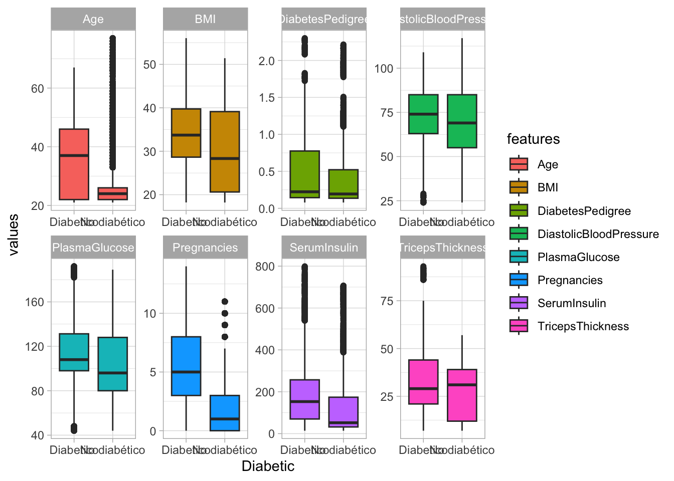
Comenzamos dividiendo los datos
# Seleccionamos 70% para entrenar (usualmente 70-80)
set.seed(2056)
diabetes_split <- diabetes %>%
  initial_split(prop = 0.70)

diabetes_train <- training(diabetes_split)
diabetes_test <- testing(diabetes_split)
Construimos el modelo:
modelo_logreg <- logistic_reg() %>%
  set_engine("glm")
Ajustamos:
logreg_fit <- modelo_logreg %>%
  fit(Diabetic ~ ., data = diabetes_train) # . significa vs todos
Checamos contra los observados:
predichos <- logreg_fit %>%
  predict(new_data = diabetes_test)

results <- diabetes_test %>%
  select(Diabetic) %>%
  bind_cols(predichos)
Midamos precisión (positive predictive value), accuracy, sensibilidad (recall), especificidad:
# Combine metrics and evaluate them all at once
eval_metrics <- metric_set(
  precision, sensitivity,
  accuracy, specificity
)
eval_metrics(data = results, truth = Diabetic, estimate = .pred_class)
# A tibble: 4 × 3
.metric .estimator .estimate
<chr> <chr> <dbl>
1 precision binary 0.754
2 sensitivity binary 0.577
3 accuracy binary 0.789
4 specificity binary 0.901También podemos sacar la matriz de confusión:
conf_mat(data = results, truth = Diabetic, estimate = .pred_class) Truth
Prediction Diabetico No diabético
Diabetico 897 293
No diabético 657 2653También podemos armar nuestra curva roc:
predice_proba <- logreg_fit %>%
  predict(new_data = diabetes_test, type = "prob")

results <- results %>%
  bind_cols(predice_proba)
results %>%
roc_curve(truth = Diabetic, .pred_Diabetico) %>%
autoplot()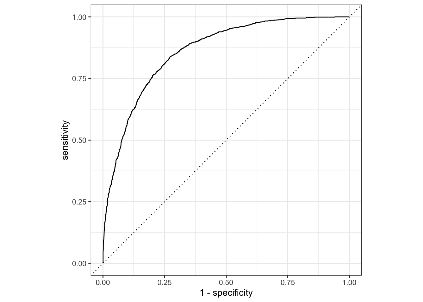
15.1 Ejercicio
- Construye tres modelos distintos para predecir diabetes sin usar la variable de glucosa (
PlasmaGlucose). Usaremos la misma basediabetesde esta sección, que ya tiene el desenlaceDiabetic(0 = no, 1 = sí):
diabedatos <- diabetes %>%
  select(-PlasmaGlucose) # quitamos la glucosa a propósito

# Así queda
dim(diabedatos)
[1] 15000 8table(diabedatos$Diabetic)
   Diabetico No diabético
        5000        10000
Nota
Este ejercicio antes usaba la base PimaIndiansDiabetes del paquete mlbench. Esa base ya no viene incluida en el paquete (la quitaron), así que la cambiamos por una que sí está disponible. Si te topas con código viejo que la usa, ahora ya sabes por qué no le funciona.
Tip
Quitar la glucosa hace el problema mucho más difícil a propósito: la glucosa es prácticamente la definición del desenlace, así que un modelo que la incluya va a predecir casi perfecto sin enseñarte nada. Lo interesante es ver cuánto se puede predecir con lo demás.
Tus modelos pueden ser logísticos pero al menos uno de los tres que sea un árbol en mode = "classification" (opciones: bart, random_forest, boost_tree, decision_tree, bag_tree)
Utiliza métricas (como sensibilidad, especificidad, etc) sobre el para decidir cuál es el mejor modelo.
16 Series de tiempo
Sección incompleta
16.1 Análisis preliminar
library(modeltime)
library(timetk)
library(lubridate)
Casos de campylobacter en Alemania (copia y pega)
library(readxl)
# Copia local. Originalmente venía del Epi R Handbook, pero esa liga ya da 404.
campylobacter_germany <- read_excel("datasets/campylobacter_germany.xlsx")
Veamos la info:
ggplot(campylobacter_germany) +
  geom_line(aes(x = date, y = case)) +
  theme_light()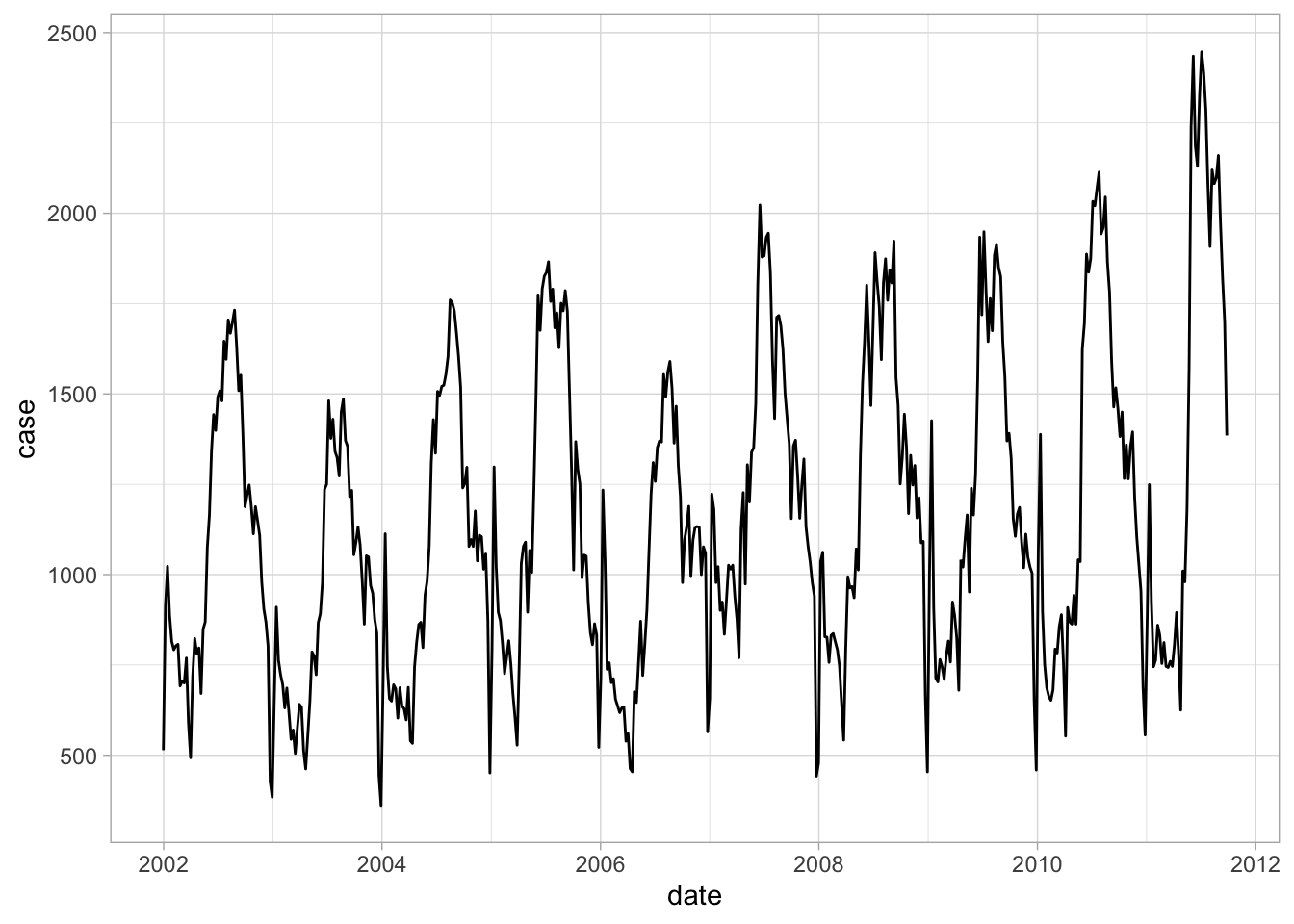
Otra forma:
campylobacter_germany %>%
  plot_time_series(date, case, .interactive = T)
Partes de una serie de tiempo clásica:
campylobacter_germany %>%
  plot_acf_diagnostics(date, case, .interactive = T, .lags = 52)
campylobacter_germany %>%
plot_seasonal_diagnostics(date, case, .interactive = T)campylobacter_germany %>%
plot_stl_diagnostics(date, case, .interactive = F)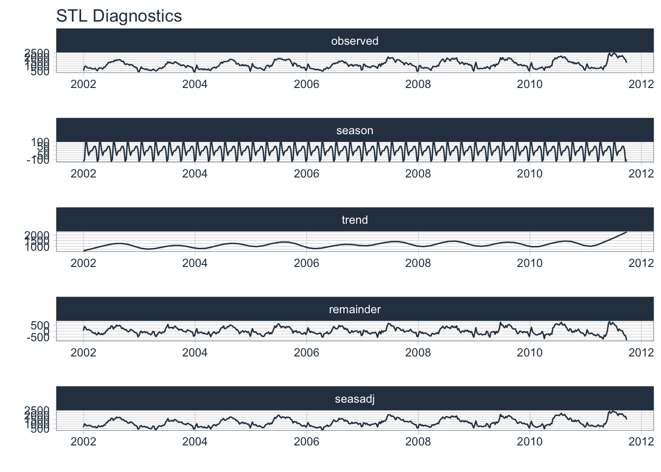
# Como no se ve completo
ggsave("Diags.pdf", width = 10, height = 25)
16.2 Modelos
En esta sección haremos arima_reg() y linear_reg(). En teoría el arima debería ser mejor que una regresión lineal.
# Para decidir el modelo primero obtenemos splits
splits <- initial_time_split(campylobacter_germany, prop = 0.8)

entrena <- training(splits)
testea <- testing(splits)

# Ajuste de un ARIMA
modelo_ARIMA <- arima_reg() %>%
  set_engine(engine = "auto_arima") %>%
  fit(case ~ date + factor(month(date, label = TRUE),
    ordered = FALSE
  ), data = entrena)

# Regresión lineal con mes como cofactor
model_lm <- linear_reg() %>%
  set_engine("lm") %>%
  fit(
    case ~ as.numeric(date) +
      factor(month(date, label = TRUE), ordered = FALSE),
    data = entrena
  )

# Junto mis modelos
models_tbl <- modeltime_table(
  modelo_ARIMA, model_lm
)

# Veo contra el test
calibration_tbl <- models_tbl %>%
  modeltime_calibrate(new_data = testea)

# Veo
calibration_tbl %>%
  modeltime_forecast(
    new_data    = testea,
    actual_data = campylobacter_germany
  ) %>%
  plot_modeltime_forecast(
    .interactive = T
  )
# Tabulo métricas
calibration_tbl %>%
modeltime_accuracy() %>%
table_modeltime_accuracy(
.interactive = T
)# Reajuste y predicción del futuro
refit_tbl <- calibration_tbl %>%
modeltime_refit(data = campylobacter_germany)
futuro <- refit_tbl %>%
modeltime_forecast(
h = "3 years",
actual_data = campylobacter_germany
)
futuro %>%
filter(.model_desc != "UPDATE: REGRESSION WITH ARIMA(3,1,0)(0,0,1)[13] ERRORS") %>%
plot_modeltime_forecast(
.interactive = T
)16.3 Ejercicio
La siguiente base de datos contiene los registros de dengue en México de 2017 a la fecha. Las variables son fecha (proxy de semana epidemológica) y nraw (casos de dengue en la semana). n es un suavizamiento con media móvil, logn y log_nraw representan los logaritmos de la media móvil n y de nraw respectivamente. Las variables t y n.value se deben ignorar.
Ajuste al menos dos modelos distintos uno de ellos
prophet_regpara determinar cuántos casos de dengue habrán hasta que termine el año.
dengue <- read_csv("https://media.githubusercontent.com/media/RodrigoZepeda/DengueMX/lognormal/datos-limpios/dengue_for_model_mx.csv") %>%
  filter(fecha >= as.Date("2017/01/01"))
17 Sistema
sessioninfo::session_info()─ Session info ───────────────────────────────────────────────────────────────
setting value
version R version 4.5.3 (2026-03-11)
os macOS Sequoia 15.7.3
system x86_64, darwin20
ui X11
language (EN)
collate es_ES.UTF-8
ctype es_ES.UTF-8
tz America/Mexico_City
date 2026-08-05
pandoc 3.10.1 @ /usr/local/bin/ (via rmarkdown)
quarto 1.10.18 @ /usr/local/bin/quarto
─ Packages ───────────────────────────────────────────────────────────────────
package * version date (UTC) lib source
abind 1.4-8 2024-09-12 [1] CRAN (R 4.5.0)
askpass 1.2.1 2024-10-04 [1] CRAN (R 4.5.0)
backports 1.5.1 2026-04-03 [1] CRAN (R 4.5.2)
base64enc 0.1-6 2026-02-02 [1] CRAN (R 4.5.1)
bayesplot 1.15.0.9000 2026-04-17 [1] https://stan-dev.r-universe.dev (R 4.5.3)
bit 4.6.0 2025-03-06 [1] CRAN (R 4.5.0)
bit64 4.8.2 2026-05-19 [1] CRAN (R 4.5.2)
boot 1.3-32 2025-08-29 [1] CRAN (R 4.5.3)
broom * 1.0.12 2026-01-27 [1] CRAN (R 4.5.1)
broom.helpers 1.22.0 2025-09-17 [1] CRAN (R 4.5.1)
cachem 1.1.0 2024-05-16 [1] CRAN (R 4.5.0)
cards 0.8.1 2026-07-06 [1] CRAN (R 4.5.2)
cellranger 1.1.0 2016-07-27 [1] CRAN (R 4.5.0)
checkmate 2.3.4 2026-02-03 [1] CRAN (R 4.5.1)
class 7.3-23 2025-01-01 [1] CRAN (R 4.5.3)
cli 3.6.6 2026-04-09 [1] CRAN (R 4.5.2)
codetools 0.2-20 2024-03-31 [1] CRAN (R 4.5.3)
colorspace 2.1-2 2025-09-22 [1] CRAN (R 4.5.1)
colourpicker 1.3.0 2023-08-21 [1] CRAN (R 4.5.0)
conflicted 1.2.0 2023-02-01 [1] CRAN (R 4.5.0)
crayon 1.5.3 2024-06-20 [1] CRAN (R 4.5.0)
crosstalk 1.2.2 2025-08-26 [1] CRAN (R 4.5.1)
curl 7.1.0 2026-04-22 [1] CRAN (R 4.5.2)
data.table 1.18.4 2026-05-06 [1] CRAN (R 4.5.2)
dials * 1.4.2 2025-09-04 [1] CRAN (R 4.5.1)
DiceDesign 1.10 2023-12-07 [1] CRAN (R 4.5.0)
digest 0.6.39 2025-11-19 [1] CRAN (R 4.5.1)
distributional 0.8.1 2026-06-27 [1] CRAN (R 4.5.2)
dplyr * 1.2.1 2026-04-03 [1] CRAN (R 4.5.2)
DT 0.34.0 2025-09-02 [1] CRAN (R 4.5.1)
dygraphs 1.1.1.6 2018-07-11 [1] CRAN (R 4.5.0)
evaluate 1.0.5 2025-08-27 [1] CRAN (R 4.5.1)
farver 2.1.2 2024-05-13 [1] CRAN (R 4.5.0)
fastmap 1.2.0 2024-05-15 [1] CRAN (R 4.5.0)
flextable * 0.9.11 2026-02-13 [1] CRAN (R 4.5.2)
fontBitstreamVera 0.1.1 2017-02-01 [1] CRAN (R 4.5.0)
fontLiberation 0.1.0 2016-10-15 [1] CRAN (R 4.5.0)
fontquiver 0.2.1 2017-02-01 [1] CRAN (R 4.5.0)
forcats * 1.0.1 2025-09-25 [1] CRAN (R 4.5.1)
forecast 9.0.2 2026-03-18 [1] CRAN (R 4.5.2)
fracdiff 1.5-3 2024-02-01 [1] CRAN (R 4.5.0)
furrr 0.3.1 2022-08-15 [1] CRAN (R 4.5.0)
future 1.70.0 2026-03-14 [1] CRAN (R 4.5.2)
future.apply 1.20.2 2026-02-20 [1] CRAN (R 4.5.2)
gdtools 0.5.0 2026-02-09 [1] CRAN (R 4.5.1)
generics 0.1.4 2025-05-09 [1] CRAN (R 4.5.0)
ggfortify * 0.4.19 2025-07-27 [1] CRAN (R 4.5.1)
ggplot2 * 4.0.3 2026-04-22 [1] CRAN (R 4.5.2)
globals 0.19.1 2026-03-13 [1] CRAN (R 4.5.2)
glue 1.8.1 2026-04-17 [1] CRAN (R 4.5.2)
gower 1.0.2 2024-12-17 [1] CRAN (R 4.5.0)
GPfit 1.0-9 2025-04-12 [1] CRAN (R 4.5.0)
gridExtra 2.3 2017-09-09 [1] CRAN (R 4.5.0)
gtable 0.3.6 2024-10-25 [1] CRAN (R 4.5.0)
gtools 3.9.5 2023-11-20 [1] CRAN (R 4.5.0)
gtsummary * 2.5.1 2026-05-30 [1] CRAN (R 4.5.2)
hardhat 1.4.2 2025-08-20 [1] CRAN (R 4.5.1)
haven * 2.5.5 2025-05-30 [1] CRAN (R 4.5.0)
hms 1.1.4 2025-10-17 [1] CRAN (R 4.5.1)
htmltools 0.5.9 2025-12-04 [1] CRAN (R 4.5.1)
htmlwidgets 1.6.4 2023-12-06 [1] CRAN (R 4.5.0)
httpuv 1.6.17 2026-03-18 [1] CRAN (R 4.5.2)
httr 1.4.8 2026-02-13 [1] CRAN (R 4.5.2)
igraph 2.2.2 2026-02-12 [1] CRAN (R 4.5.2)
infer * 1.1.0 2025-12-18 [1] CRAN (R 4.5.1)
inline 0.3.21 2025-01-09 [1] CRAN (R 4.5.0)
ipred 0.9-15 2024-07-18 [1] CRAN (R 4.5.0)
janitor 2.2.1 2024-12-22 [1] CRAN (R 4.5.0)
jsonlite 2.0.0 2025-03-27 [1] CRAN (R 4.5.0)
knitr 1.51 2025-12-20 [1] CRAN (R 4.5.1)
labeling 0.4.3 2023-08-29 [1] CRAN (R 4.5.0)
labelled 2.16.0 2025-10-22 [1] CRAN (R 4.5.1)
later 1.4.8 2026-03-05 [1] CRAN (R 4.5.2)
lattice 0.22-9 2026-02-09 [1] CRAN (R 4.5.3)
lava 1.8.2 2025-10-30 [1] CRAN (R 4.5.1)
lhs 1.2.1 2026-03-01 [1] CRAN (R 4.5.2)
lifecycle 1.0.5 2026-01-08 [1] CRAN (R 4.5.1)
listenv 0.10.1 2026-03-10 [1] CRAN (R 4.5.2)
lme4 2.0-6 2026-07-16 [1] CRAN (R 4.5.2)
loo 2.10.0.9000 2026-07-10 [1] https://stan-dev.r-universe.dev (R 4.5.3)
lubridate * 1.9.5 2026-02-04 [1] CRAN (R 4.5.1)
magrittr 2.0.5 2026-04-04 [1] CRAN (R 4.5.2)
markdown 2.0 2025-03-23 [1] CRAN (R 4.5.0)
MASS 7.3-65 2025-02-28 [1] CRAN (R 4.5.3)
Matrix 1.7-5 2026-03-21 [1] CRAN (R 4.5.2)
matrixStats 1.5.0 2025-01-07 [1] CRAN (R 4.5.0)
memoise 2.0.1 2021-11-26 [1] CRAN (R 4.5.0)
mime 0.13 2025-03-17 [1] CRAN (R 4.5.0)
miniUI 0.1.2 2025-04-17 [1] CRAN (R 4.5.0)
minqa 1.2.8 2024-08-17 [1] CRAN (R 4.5.0)
modeldata * 1.5.1 2025-08-22 [1] CRAN (R 4.5.1)
modeltime * 1.3.5 2026-01-31 [1] CRAN (R 4.5.1)
nlme 3.1-168 2025-03-31 [1] CRAN (R 4.5.3)
nloptr 2.2.1 2025-03-17 [1] CRAN (R 4.5.0)
nnet 7.3-20 2025-01-01 [1] CRAN (R 4.5.3)
officer 0.7.3 2026-01-16 [1] CRAN (R 4.5.1)
openssl 2.4.2 2026-06-09 [1] CRAN (R 4.5.2)
otel 0.2.0 2025-08-29 [1] CRAN (R 4.5.1)
palmerpenguins * 0.1.1 2022-08-15 [1] CRAN (R 4.5.0)
parallelly 1.47.0 2026-04-17 [1] CRAN (R 4.5.2)
parsnip * 1.4.1 2026-01-11 [1] CRAN (R 4.5.1)
patchwork 1.3.2 2025-08-25 [1] CRAN (R 4.5.1)
pillar 1.11.1 2025-09-17 [1] CRAN (R 4.5.1)
pkgbuild 1.4.8 2025-05-26 [1] CRAN (R 4.5.0)
pkgconfig 2.0.3 2019-09-22 [1] CRAN (R 4.5.0)
plotly 4.12.1 2026-07-22 [1] CRAN (R 4.5.2)
plyr 1.8.9 2023-10-02 [1] CRAN (R 4.5.0)
poissonreg * 1.0.2 2026-04-20 [1] CRAN (R 4.5.2)
posterior 1.7.1 2026-07-15 [1] https://stan-dev.r-universe.dev (R 4.5.3)
prodlim 2026.03.11 2026-03-11 [1] CRAN (R 4.5.2)
promises 1.5.0 2025-11-01 [1] CRAN (R 4.5.1)
purrr * 1.2.2 2026-04-10 [1] CRAN (R 4.5.2)
QuickJSR 1.10.0 2026-05-17 [1] CRAN (R 4.5.2)
R6 2.6.1 2025-02-15 [1] CRAN (R 4.5.0)
ragg 1.5.2 2026-03-23 [1] CRAN (R 4.5.2)
rbibutils 2.4.1 2026-01-21 [1] CRAN (R 4.5.1)
RColorBrewer 1.1-3 2022-04-03 [1] CRAN (R 4.5.0)
Rcpp * 1.1.2 2026-07-05 [1] CRAN (R 4.5.2)
RcppParallel 5.1.11-2 2026-03-05 [1] CRAN (R 4.5.2)
Rdpack 2.6.6 2026-02-08 [1] CRAN (R 4.5.1)
reactable 0.4.5 2025-12-01 [1] CRAN (R 4.5.1)
reactR 0.6.1 2024-09-14 [1] CRAN (R 4.5.0)
readr * 2.2.0 2026-02-19 [1] CRAN (R 4.5.2)
readxl * 1.4.5 2025-03-07 [1] CRAN (R 4.5.0)
recipes * 1.3.1 2025-05-21 [1] CRAN (R 4.5.0)
reformulas 0.4.4 2026-02-02 [1] CRAN (R 4.5.1)
reshape2 1.4.5 2025-11-12 [1] CRAN (R 4.5.1)
rlang 1.3.0 2026-07-05 [1] CRAN (R 4.5.2)
rmarkdown 2.31 2026-03-26 [1] CRAN (R 4.5.2)
rpart 4.1.24 2025-01-07 [1] CRAN (R 4.5.3)
rsample * 1.3.2 2026-01-30 [1] CRAN (R 4.5.1)
rstan 2.36.0.9000 2026-05-22 [1] https://stan-dev.r-universe.dev (R 4.5.3)
rstanarm * 2.32.2 2025-09-30 [1] CRAN (R 4.5.1)
rstantools 2.6.0.9000 2026-01-10 [1] https://stan-dev.r-universe.dev (R 4.5.3)
rstudioapi 0.19.0 2026-06-11 [1] CRAN (R 4.5.2)
S7 0.2.2 2026-04-22 [1] CRAN (R 4.5.2)
scales * 1.4.0 2025-04-24 [1] CRAN (R 4.5.0)
sessioninfo 1.2.3 2025-02-05 [1] CRAN (R 4.5.0)
shiny 1.13.0 2026-02-20 [1] CRAN (R 4.5.2)
shinyjs 2.1.1 2026-01-15 [1] CRAN (R 4.5.1)
shinystan 2.7.0 2025-12-12 [1] CRAN (R 4.5.1)
shinythemes 1.2.0 2021-01-25 [1] CRAN (R 4.5.0)
snakecase 0.11.1 2023-08-27 [1] CRAN (R 4.5.0)
sparsevctrs 0.3.6 2026-01-27 [1] CRAN (R 4.5.1)
StanHeaders 2.36.0.9000 2026-05-22 [1] https://stan-dev.r-universe.dev (R 4.5.3)
stringi 1.8.7 2025-03-27 [1] CRAN (R 4.5.0)
stringr * 1.6.0 2025-11-04 [1] CRAN (R 4.5.1)
survival 3.8-6 2026-01-16 [1] CRAN (R 4.5.3)
systemfonts 1.3.2 2026-03-05 [1] CRAN (R 4.5.2)
tailor * 0.1.0 2025-08-25 [1] CRAN (R 4.5.1)
tensorA 0.36.2.1 2023-12-13 [1] CRAN (R 4.5.0)
textshaping 1.0.5 2026-03-06 [1] CRAN (R 4.5.2)
threejs 0.3.4 2025-04-21 [1] CRAN (R 4.5.0)
tibble * 3.3.1 2026-01-11 [1] CRAN (R 4.5.1)
tidymodels * 1.4.1 2025-09-08 [1] CRAN (R 4.5.1)
tidyr * 1.3.2 2025-12-19 [1] CRAN (R 4.5.1)
tidyselect 1.2.1 2024-03-11 [1] CRAN (R 4.5.0)
tidyverse * 2.0.0 2023-02-22 [1] CRAN (R 4.5.0)
timechange 0.4.0 2026-01-29 [1] CRAN (R 4.5.1)
timeDate 4052.112 2026-01-28 [1] CRAN (R 4.5.1)
timetk * 2.9.1 2025-08-29 [1] CRAN (R 4.5.1)
tune * 2.0.1 2025-10-17 [1] CRAN (R 4.5.1)
tzdb 0.5.0 2025-03-15 [1] CRAN (R 4.5.0)
urca 1.3-4 2024-05-27 [1] CRAN (R 4.5.0)
utf8 1.2.6 2025-06-08 [1] CRAN (R 4.5.0)
uuid 1.2-2 2026-01-23 [1] CRAN (R 4.5.1)
V8 8.2.0 2026-04-21 [1] CRAN (R 4.5.2)
vctrs 0.7.3 2026-04-11 [1] CRAN (R 4.5.2)
viridisLite 0.4.3 2026-02-04 [1] CRAN (R 4.5.1)
vroom 1.7.1 2026-03-31 [1] CRAN (R 4.5.2)
withr 3.0.3 2026-06-19 [1] CRAN (R 4.5.2)
workflows * 1.3.0 2025-08-27 [1] CRAN (R 4.5.1)
workflowsets * 1.1.1 2025-05-27 [1] CRAN (R 4.5.0)
xfun 0.60 2026-07-09 [1] CRAN (R 4.5.2)
xml2 1.6.0 2026-06-22 [1] CRAN (R 4.5.2)
xtable 1.8-8 2026-02-22 [1] CRAN (R 4.5.2)
xts 0.14.2 2026-02-28 [1] CRAN (R 4.5.2)
yaml 2.3.12 2025-12-10 [1] CRAN (R 4.5.1)
yardstick * 1.3.2 2025-01-22 [1] CRAN (R 4.5.0)
zip 3.0.1 2026-07-13 [1] CRAN (R 4.5.2)
zoo 1.8-15 2025-12-15 [1] CRAN (R 4.5.1)
[1] /Library/Frameworks/R.framework/Versions/4.5-x86_64/Resources/library
* ── Packages attached to the search path.
──────────────────────────────────────────────────────────────────────────────