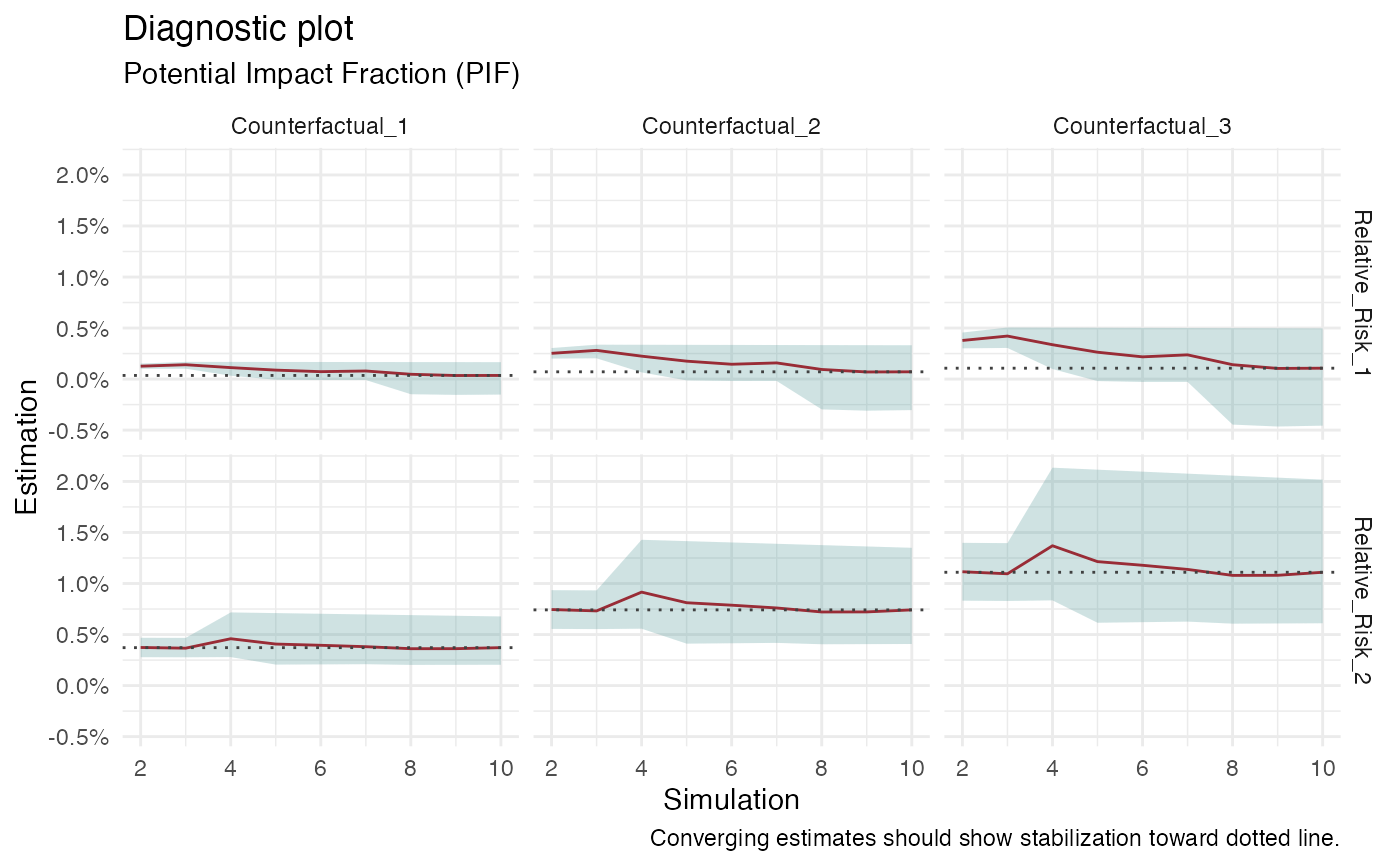
Diagnostic bootstrap plots for pif_class — diagnostic

Creates a ggplot2::ggplot() object containing diagnostic plots for the convergence of the population attributable fraction and potential impact fraction

Usage

diagnostic_plot(x, relative_risks = NULL, counterfactuals = NULL, level = 0.95)

Arguments

x: A pif_class object
relative_risks: Vector of relative risk names to plot (set to NULL to plot all)
counterfactuals: Vector of counterfactual names to plot (set to NULL to plot all)
level: (double) Level for the quantiles of the plot (default to 0.95)

Value

A ggplot2 object with caterpillar plots to assess convergence

Examples

# EXAMPLE 1
# Setup the survey design
data(ensanut)
options(survey.lonely.psu = "adjust")
design <- survey::svydesign(data = ensanut, ids = ~1, weights = ~weight, strata = ~strata)

# Calculate two different relative risks
rr <- list(
 function(X, theta) {exp(theta[1] * X[, "systolic_blood_pressure"] / 100)},
 function(X, theta) {exp(theta[2] * X[, "systolic_blood_pressure"] / 100 + theta[3]* X[,"age"])}
)

# Calculate three counterfactual scenarios of SBP reduction from 1 to 3 mmhg
cft <- list(
function(X){X[, "systolic_blood_pressure"]  <- X[, "systolic_blood_pressure"]  - 1; return(X)},
function(X){X[, "systolic_blood_pressure"]  <- X[, "systolic_blood_pressure"]  - 2; return(X)},
function(X){X[, "systolic_blood_pressure"]  <- X[, "systolic_blood_pressure"]  - 3; return(X)}
)

my_pif <- pif(design,
  theta = log(c(1.05, 1.38, 1.21)), rr, cft,
  additional_theta_arguments = c(0.01, 0.03, 0.025),
  n_bootstrap_samples = 10,
)
diagnostic_plot(my_pif)