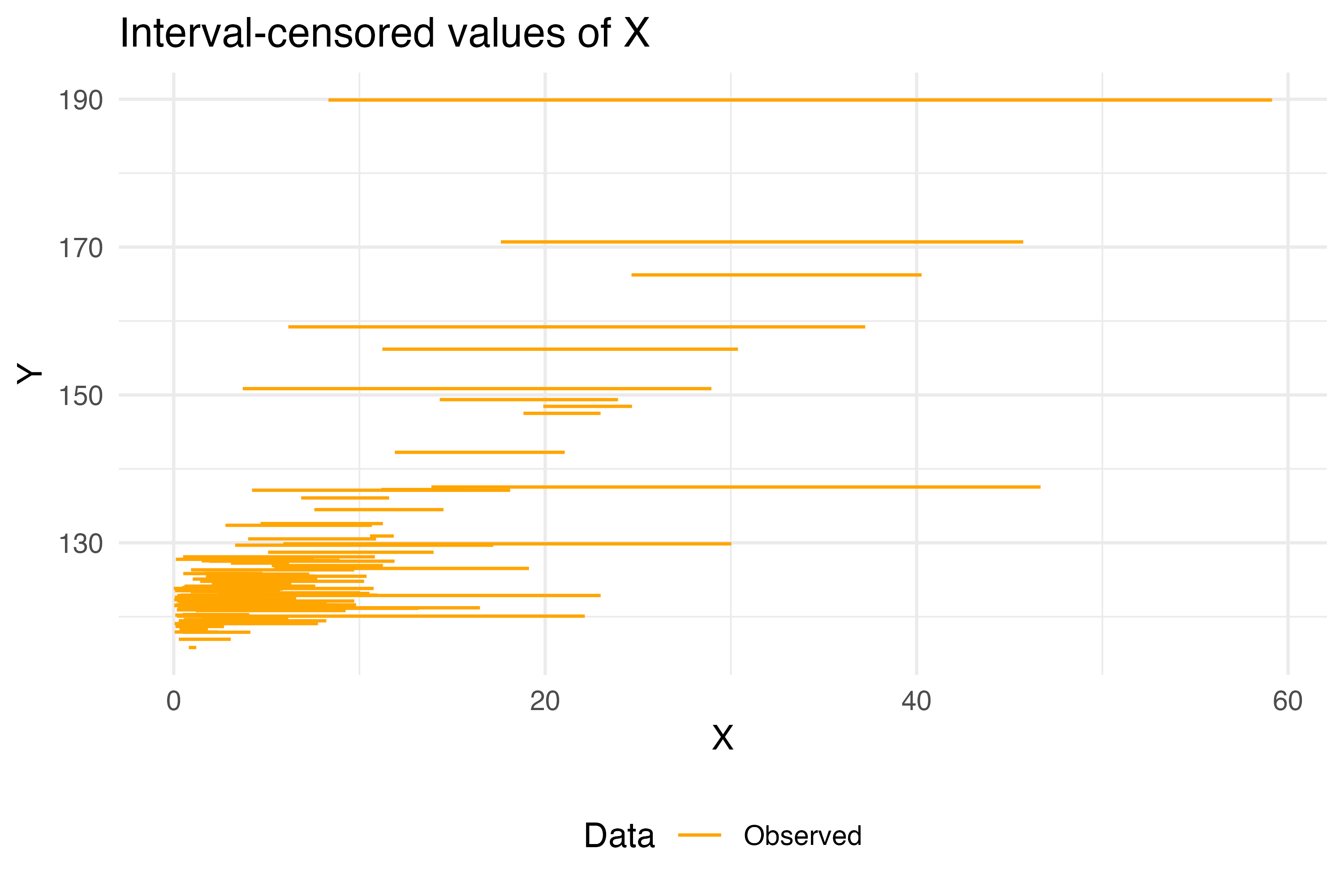
Bayesian interval regression with `Stan`

Stan

Bayesian

Regression

cmdstanr

statistics

Author

Rodrigo Zepeda-Tello

Published

March 9, 2024

Abstract

In this entry I discuss how to do a linear regression model when the dependent variable is represented as an interval. That is, when we only know ranges for \(X\) and we know there is a linear association between \(X\) and \(Y\).

The problem

Consider the following problem where we have measurements for the response variable \(Y\) and interval-valued dependent \(X\). As an example problem we can think of \(X\) as consumption levels for a nutrient (grams per day) and \(Y\) can be an outcome (systolic blood pressure). An example database would be as follows:

X	Y
factor	numeric
(1,3]	123.7
(5,10]	132.6
(1,3]	120.1
(3,5]	125.7
[0,1]	115.8
(1,3]	128.2
(1,3]	122.9
(10,Inf]	141.5
(1,3]	117.8
[0,1]	123.8
n: 100

To solve this we’ll first review the classical formulation, then the interval-valued formulation and finally we’ll program it in Stan.

Classical model

A classical Bayesian linear regression model (if the complete \(X\) was observed) is given by: \[\begin{equation} Y|_{X = x} \sim \textrm{Normal}(\beta_0 + \beta_1 x, \sigma^2) \end{equation}\] with priors for the parameters: \[\begin{equation} \beta_0 \sim \textrm{Normal}(0,100), \quad \beta_1 \sim \textrm{Normal}(0,100), \quad \sigma \sim \textrm{Normal}_+(0,100). \end{equation}\]

written in terms of the likelihood is re presented as: \[\begin{equation} \begin{aligned} \mathcal{L}(\beta_0, \beta_1, \sigma | x, y) & \propto p(y,x | \beta_0,\beta_1,\sigma)\cdot p(\beta_0,\beta_1, \sigma) \\ & \propto p(y|x, \beta_0,\beta_1,\sigma) \cdot p(\beta_0,\beta_1, \sigma) \end{aligned} \end{equation}\]

This term assumes \(X\) is a constant and hence there is no need to specify a prior on \(X\) nor to include the term \(p(x| \beta_0,\beta_1,\sigma)\) in the likelihood. When \(X\) is considered a random variable, the distribution of \(X\) (say \(f_X\)) is included as a prior and in the likelihood too:

\[\begin{equation} X \sim f_ X\quad \text{and} \quad Y|_{X = x} \sim \textrm{Normal}(\beta_0 + \beta_1 x, \sigma^2) \end{equation}\]

and identical priors for the parameters.

The likelihood now includes a term for \(X\): \[\begin{equation} \begin{aligned} \mathcal{L}(\beta_0, \beta_1, \sigma | x, y) & \propto p(y,x | \beta_0, \beta_1, \sigma) \cdot p(\beta_0, \beta_1, \sigma) \\ & \propto p(y|x, \beta_0,\beta_1,\sigma) \cdot p(x| \beta_0,\beta_1,\sigma)\cdot p(\beta_0,\beta_1, \sigma). \end{aligned} \end{equation}\]

Usually, \(X\) is independent from \(\beta_0,\beta_1\) and \(\sigma\) hence we can write \(p(x| \beta_0,\beta_1,\sigma) = p(x)\):

\[\begin{equation}\label{eqlike} \mathcal{L}(\beta_0, \beta_1, \sigma | x, y) \propto p(y|x, \beta_0,\beta_1,\sigma)\cdot p(x) \cdot p(\beta_0,\beta_1, \sigma). \end{equation}\]

Programming this in Stan

We’ll start with this model with a lognormal distribution for \(X\) as an example:

\[\begin{equation} X \sim \textrm{Lognormal}(\mu, \tau) \quad \text{and} \quad Y|_{X = x} \sim \textrm{Normal}(\beta_0 + \beta_1 x, \sigma^2) \end{equation}\]

and priors: \[\begin{equation} \beta_0 \sim \textrm{Normal}(0,100), \quad \beta_1 \sim \textrm{Normal}(0,100), \quad \sigma \sim \textrm{Normal}_+(0,100) \quad \tau \sim \textrm{Normal}_+(0,100). \end{equation}\]

The stan code is given by:

data {
  int<lower=1> N;       //Total sample size
  vector<lower=0>[N] X; //Observed X-values
  vector[N] Y;          //Observed Y-values
}

parameters {
  //Mean parameter of X
  real<lower=0> mu;
  
  //Parameters for regression
  real beta_0;
  real beta_1;
  
  //Parameters for variance
  real<lower=0> sigma;
  real<lower=0> tau;
}

transformed parameters {
  vector[N] y_mean = rep_vector(beta_0, N) + beta_1*X;
}

model {
  beta_0 ~ normal(0, 100);
  beta_1 ~ normal(0, 100);
  sigma  ~ normal(0, 100);
  tau    ~ normal(0, 100);
  X      ~ lognormal(mu, tau);
  Y      ~ normal(y_mean, sigma);
}

you can save it into a file called regression_linear.stan and fit the model

#Install cmdstanr from their website
#https://mc-stan.org/cmdstanr/
library(cmdstanr)
library(tidybayes)
set.seed(274865)

#Create an example dataset
nsamples <- 100
beta_0   <- 120
beta_1   <- 1.2
sigma_y  <- 2
mu_x     <- 1
tau_x    <- 1.4

example_db <- tibble(
  Xtrue = rlnorm(nsamples, meanlog = mu_x, sdlog = tau_x), 
  Y     = beta_0 + beta_1*Xtrue + rnorm(nsamples, sd = sigma_y)
)

stan_data <- list(
  N = nrow(example_db),
  X = example_db$Xtrue,
  Y = example_db$Y
)

#Compile the model
model_1 <- cmdstan_model("regression_linear.stan")

#And fit
fit_model <- model_1$sample(
   data = stan_data,
   seed = 4275,
   chains = 4,
   parallel_chains = 4,
   refresh = 0
)

The results are very close to the true values:

#We can then verify that the fitted values are very close to the true values
fit_model |> 
  summarise_draws() |> 
  filter(variable %in% c("beta_0","beta_1","sigma","tau","mu")) |> 
  as_flextable()

variable	mean	median	sd	mad	q5	q95	rhat	ess_bulk	ess_tail
character	numeric	numeric	numeric	numeric	numeric	numeric	numeric	numeric	numeric
mu	0.7	0.7	0.1	0.1	0.5	1.0	1.0	3,679.4	2,064.2
beta_0	119.9	119.9	0.2	0.2	119.5	120.3	1.0	3,813.0	3,135.5
beta_1	1.2	1.2	0.0	0.0	1.2	1.2	1.0	4,488.7	2,759.6
sigma	2.1	2.1	0.2	0.2	1.9	2.4	1.0	4,979.6	2,797.9
tau	1.5	1.5	0.1	0.1	1.3	1.7	1.0	4,420.0	2,885.7
n: 5

Interval-censored model

We now consider the case where \(X\) is not observed completely but only the ranges of \(X\). Survival analysis theory considers three types of ranges:

Right censored: Correspond to values where we only know the lower bound: \([a,\infty]\).
Left censored: Are intervals where only the upper bound is known: \([-\infty, b]\).
Interval censored: Are ranges of \(X\) in the shape \([a,b]\) where \(a,b\) are real numbers.

For our example, we’ll consider the following dataset where the unknown X is in the range between X_low and X_up. So, this example is only for interval-censored data¹.

example_problem <- 
  tibble(Xtrue = rlnorm(nsamples, meanlog = mu_x, sdlog = tau_x), 
         Y     = beta_0 + beta_1*Xtrue + rnorm(nsamples, sd = sigma_y), 
         X_low = runif(nsamples, 0, Xtrue),
         X_up  = Xtrue + rlnorm(nsamples, meanlog = 1, sdlog = 1)
  ) |> 
  select(X_low, X_up, Y)
  
as_flextable(example_problem)

X_low	X_up	Y
numeric	numeric	numeric
1.1	2.0	119.4
0.1	0.8	120.6
1.3	7.8	128.2
3.4	8.2	124.8
1.6	4.5	123.0
0.2	2.9	118.3
1.0	2.3	121.9
0.5	2.8	123.3
6.5	11.0	128.3
2.0	6.0	122.5
n: 100

In this case, the likelihood needs to account for the fact that the conditional probability is now for an interval and the conditional joint distribution is required:

\[\begin{equation} \begin{aligned} \mathcal{L}(\beta_0, \beta_1, \sigma | x \in [a,b], y) & \propto p(y,x \in [a,b] | \beta_0,\beta_1,\sigma) \cdot p(\beta_0,\beta_1, \sigma) \\ & \propto \left[\int\limits_{a}^{b} p(y | x, \beta_0,\beta_1,\sigma) p(x) dx\right] \cdot p(\beta_0,\beta_1, \sigma) \end{aligned} \end{equation}\]

we can program this in Stan by creating this part of the likelihood function separately. Here I’m first summing the log-likelihoods and then exponentiating for numerical stability of the integration process.

functions {
  // Lognormal probability density function
  real log_lognormal_pdf(real x, real mu_lognormal, real sigma_lognormal) {
    //1/(1 / (x * sigma * sqrt(2 * pi())) * exp(- 0.5*((log(x) - mu)/sigma)^2)
    
    //Values for logarithm.
    real log_x = log(x);

    //This corresponds to log(1 / (x * sigma * sqrt(2 * pi())))
    //The constant is removed as Bayes only requires proportionality
    real log_normalization = -(log_x + log(sigma_lognormal));
    
    //Exponent of the lognormal
    real exponent = -0.5*square((log_x - mu_lognormal) / sigma_lognormal);
    
    //For numerical stability sum in log-scale
    return log_normalization + exponent;
  }
  
  // Normal probability density function
  real log_normal_pdf(real y, real mu, real sigma) {
    //1/(1 / (sqrt(2 * pi())*sigma) * exp(- 0.5*((x - mu)/sigma)^2)
    
    //Normal density without the 2*pi as Bayes requires only proportionality
    real log_normalization = -log(sigma);
    real log_exponent      = -0.5 * square((y - mu) / sigma);

    return log_normalization + log_exponent;
  }
  
  real integrand_pdf(real x, real xc, array[] real theta, array[] real x_r, array[] int x_i) {
    //Linear model
    real mu  = theta[4] + theta[5]*x;
    
    //Return the exponential of the log sum
    return exp(log_lognormal_pdf(x, theta[2], theta[3]) + log_normal_pdf(x_r[1], mu, theta[1]));
  }
}

We then construct the likelihood in Stan (file regression_interval.stan) using the integrate_1d routine with a precision of \(\epsilon^{2/3}\) as suggested by the Boost website:

#include integrand.stan

data {
  int<lower=1> N;           //Total sample size
  vector<lower=0>[N] X_low; //Observed lower bound for X
  vector<lower=0>[N] X_up;  //Observed upper bound for X
  vector[N] Y;              //Observed Y-values
}


transformed data {
  //Normalize Y to help inference process
  real mu_Y = mean(Y);
  real sigma_Y = sd(Y);
  vector[N] y_centered = (Y - mu_Y)/sigma_Y;
  
  //Required for integration
  array[0] int x_i;
}

parameters {
  //Mean parameter of X
  real<lower=0> mu;
  
  //Parameters for regression
  real beta_0;
  real beta_1;
  
  //Parameters for variance
  real<lower=0> sigma;
  real<lower=0> tau;
}

model {
  beta_0 ~ normal(0, 100);
  beta_1 ~ normal(0, 100);
  sigma  ~ normal(0, 100);
  tau    ~ normal(0, 100);
  
  //Add the likelihood for intervals
  for (i in 1:N){
    target += log(integrate_1d(
      integrand_pdf, X_low[i], X_up[i], 
        {sigma, mu, tau, beta_0, beta_1}, {y_centered[i]}, x_i,
        pow(machine_precision(), 0.25))
    );
  }
}

generated quantities {
  real beta_0_real = sigma_Y*beta_0 + mu_Y;
  real beta_1_real = sigma_Y*beta_1;
  real sigma_real  = sigma_Y*sigma;
}

Finally, the R code to infer the parameters which result good estimations of the true values.

#Install cmdstanr from their website
#https://mc-stan.org/cmdstanr/
model_2 <- cmdstan_model("regression_interval.stan")

stan_data <- list(
  N     = nrow(example_problem),
  X_low = example_problem$X_low,
  X_up  = example_problem$X_up,
  Y     = example_problem$Y
)

#And fit
fit_model <- model_2$sample(
  data = stan_data,
  seed = 4275,
  chains = 1,
  parallel_chains = 1,
  #refresh = 0
)

#We can then verify that the fitted values are very close to the true values
fit_model |> 
  summarise_draws() |> 
  filter(variable %in% c("beta_0_real","beta_1_real","sigma_real","tau","mu")) |> 
  as_flextable()

variable	mean	median	sd	mad	q5	q95	rhat	ess_bulk	ess_tail
character	numeric	numeric	numeric	numeric	numeric	numeric	numeric	numeric	numeric
mu	1.2	1.2	0.1	0.1	1.0	1.4	1.0	972.6	583.6
tau	1.1	1.1	0.1	0.1	0.9	1.2	1.0	1,002.1	659.7
beta_0_real	118.6	118.6	0.3	0.4	118.0	119.1	1.0	669.6	645.5
beta_1_real	1.4	1.4	0.1	0.1	1.3	1.5	1.0	778.2	613.0
sigma_real	1.9	1.8	0.2	0.2	1.6	2.2	1.0	1,261.1	720.2
n: 5

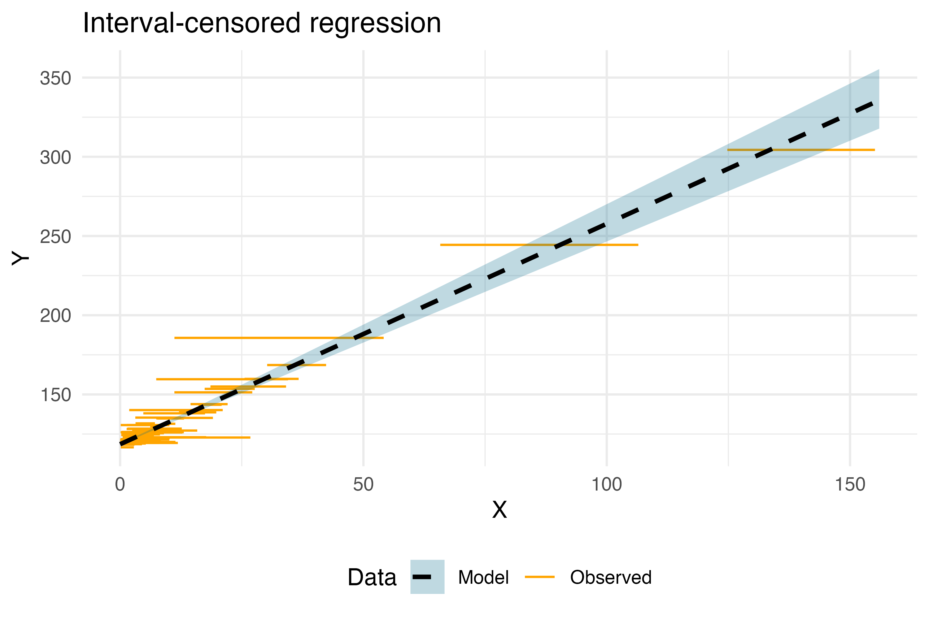
Which, graphically, results in the following regression model:

Show code for plot

draws_model <- fit_model$draws(format = "draws_df")
for (k in 0:ceiling(max(example_problem$X_up))){
  temp <- draws_model |> 
    mutate(X = !!k) |> 
    mutate(Y = beta_0_real + beta_1_real*X) |> 
    summarise(
      Yval = mean(Y),
      q025 = quantile(Y, 0.025),
      q975 = quantile(Y, 0.975),
    ) |> 
    mutate(
      X = !!k
    )
  
  if (k == 0){
    results_model <- temp
  } else {
    results_model <- results_model |> bind_rows(temp)
  }
  
}

plt <- ggplot(example_problem) +
  geom_segment(aes(x = X_low, xend = X_up, y = Y, yend = Y, 
                   color = "Observed", fill = "Observed")) +
  geom_ribbon(aes(x = X, ymin = q025, ymax = q975, 
                  fill = "Model"), data = results_model, alpha = 0.25) + 
  geom_line(aes(x = X, y = Yval, color = "Model"), data = results_model, linewidth = 1,
            linetype = "dashed") + 
  theme_minimal() +
  labs(
    x = "X",
    y = "Y",
    title = "Interval-censored regression"
  ) +
  scale_color_manual("Data", values = c("Model" = "black", "Observed" = "orange")) +
  scale_fill_manual("Data", values = c("Model" = "deepskyblue4", "Observed" = "orange")) +
  theme(legend.position = "bottom")
ggsave("Interval.png", width = 6, height = 4, dpi = 500, plot = plt)

Discusion

This is, of course, not the only way to do this model. A different approach would be to assume that the true \(X\) restricted to the interval \([a,b]\) has a certain distribution (for example, a Uniform). I find this approach useful (for convergence) but not so intuitive for the priors. Let me know if you’d like a tutorial on this different approach.

Footnotes

Extensions to right/left can be done including more ifs and using Stan’s special values of positive_infinity() and negative_infinity().↩︎